PROCESS IN NORTH AMERICAN FREIGHT RAILROADS. Rainer Guttkuhn .... Train arrivals (resulting in the crew tie-up at the arrival terminal, the ...
Proceedings of the 2003 Winter Simulation Conference S. Chick, P. J. Sánchez, D. Ferrin, and D. J. Morrice, eds.
A DISCRETE EVENT SIMULATION FOR THE CREW ASSIGNMENT PROCESS IN NORTH AMERICAN FREIGHT RAILROADS Rainer Guttkuhn Todd Dawson Udo Trutschel
Jon Walker Mike Moroz Canadian National Railroad Edmonton, Alberta T5J 0K2, CANADA
24 Hartwell Avenue Circadian Technologies, Inc. Lexington, MA 02421, U.S.A.
ing, gotten more attention by using discrete event simulations as assessment tools (Dalal 2001). Freight railroads in North America traditionally assign crews to trains by means of maintaining a board of crews at one or more local crew points. Crews usually move trains between two terminals, their home terminal (HT) and a designated away-from-home terminal (AFHT). Crews are called from the top of the board and added to the bottom of the board when they become available for call again upon returning home. All crews cycle through such a board at their HT and their AFHT. For each train a decision has to be made what board to call a crew from; Is it better to send a new home crew out on a particular train or to send an AFHT crew home on a particular train? Often the portion of the traffic that has to be assigned to one terminal (workload allocation or equity) is determined by labor agreements and has to be observed within small margins. Each of those assignment decisions results in a different subset of trains and a different setup of the crew boards. These factors have consequences for subsequent crew assignment options and the overall operational performance. The problem is too complex to calculate a mathematical solution for assessing the operational performance of certain combinations of traffic, rules and different crew assignment scenarios by hand. Only a computer simulation can provide meaningful answers to these what-if questions. As part of a co-development project between CN Rail and Circadian Technologies, Inc., a simulation module called ‘TrainSim’ was created that simulates the crew assignment process. The program is written in Delphi 6.0, runs on the MS 32bit Windows platform and connects to a local Paradox database for retrieval of parameters, rules, train traffic, crew schedules and the storage of the resulting crew assignments.
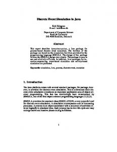
ABSTRACT This paper introduces a discrete event simulation for crew assignments and crew movements as a result of train traffic, labor rules, government regulations and optional crew schedules. The software is part of a schedule development system, FRCOS (Freight Rail Crew Optimization System), that was co-developed by Canadian National (CN) Rail and Circadian Technologies, Inc. The simulation allows verification of the impact of changes to trainflow, labor rules or government regulations on the overall operational efficiency of how crews are called to work. The system helps to evaluate changes to current crew assignments and can test new crew assignment scenarios such as crew schedules. Potential problems can be detected before the actual implementation, saving unnecessary costs. The software is also used to assess the impact of traffic changes on existing crew schedules in order to implement reactive corrections to these schedules. 1
INTRODUCTION
A growing number of transportation firms are utilizing discrete event simulations to model the various conditions of their operations (Banks 1998). Some typical topics for the application of simulation tools in the North American Railroads include loading strategies at the rail yards, train timetables, capacity requirements for train cars, locomotive utilization and track availability. In general the simulation techniques are used for the evaluation of strategies designed to improve the operational performance of equipment (Homer et. al. 1999). In most of the current railroad operations crews are required to be on call 24 hours a day, 7 days a week. This results in highly irregular work patterns, high fatigue and constant uncertainty in personal and family life. Only in the last few years have the operational, physiological and social impact of different crew assignment scenarios, including crew schedul-
1686
Guttkuhn, Dawson, Trutschel, Walker, and Moroz 2
TRAINSIM - SIMULATION GOALS
•
TrainSim allows the user to answer operational “what-if” questions in a very efficient way, without disturbing the real railroad operation. The simulation engine provides a sophisticated replication of the crew assignment process as a function of time and specified operational parameters, creating a prediction of the results of particular crew assignments based on historical or fabricated train flow. The results of the simulation allow the user to draw conclusions concerning the operational characteristics of the real crew assignment process. The TrainSim software stores the results of the simulation in a database, which allows for extensive analysis of operational, sociological, and physiological parameters. This information provides the basis for answering the “what if” questions posed in the simulation. The following list outlines benefits and suggested uses for the simulator: • Quickly assess changes in the crew assignment process. This is critical, because once a selected crew assignment implementation has been started in the real operation, changes and corrections can be extremely expensive. The simulator allows the user to view the resulting increase or decrease in pool costs that result from varying particular parameters in the simulation. The speed of the simulation also provides near-real time assessments of changes in traffic patterns on crew assignments. • Determine the level of detail. Using a comprehensive set of data filters, the user can statistically examine the overall crew management process of a whole year in minutes or spend several hours examining specific events that occurred during the crew assignment process. • Explore possibilities. Potential new policies and operational rules can be simulated without disrupting the operation of the real system. The effects of parameter variations on crew assignment performance can be explored and potential associated cost increases or decreases can be determined to provide the basis for accepting or implementing new changes to crew assignment. • Diagnose problems. With the help of the simulation, all aspects of the operation can be investigated on a detailed level. The speed of the software allows the user to examine many parameters quickly and make appropriate adjustments. For example, changes to service design regarding scheduled and/or modular trains train schedules and their impact on existing or proposed crew schedules can be evaluated. In addition, excessive crew fatigue can be detected and methods for fatigue mitigation explored.
•
•
•
•
1687
Identify constraints and bottlenecks. Since the simulation can simulate any type of crew schedule based on time of availability, including simple days-on-days-off patterns, it allows the determination of the number and positioning of days on/off which can be scheduled without creating potential crew shortages. The software can also help determine the impact of temporary changes to train operations due to work programs or service disruptions. Develop understanding and build consensus. The easy-to-read and quickly accessible charts and tables generated by the software make it a tool for sharing information among many different groups in a real-time manner. The software also provides tangible data that is objective and impartial. This feature is invaluable when evaluating the various suggestions and changes and determining the impact of the changes and associated cost increases or decreases. Simulations of varying parameters help all who are involved in scheduling to understand the impact of changes to crew utilization on both the overall operation and the crews themselves. Prepare for change. It is clear that some form of crew scheduling is in the future for railroads. However, not all operations can work the same type of crew scheduling system. Determining the optimal scheduling methodology and answering all the “what-if” questions are useful for designing new crew assignments that have the best fit of operational, sociological, and physiological parameters for a specific operation. The detailed analyses of the simulation reporting system provide the proper tools for testing and evaluating all the possible scenarios for scheduling crews in any operation. Train the crew management team. One example would be to show crew callers the consequences of certain calls, including the complex interaction between calling a crew from a pool or the extraboard. It also assists in determining the impact of different calling procedures on the operation of the overall pool as well as the impact on specific crews. Predict appropriate staffing levels of pool and extraboard as a function of time. This is important because overstaffing is costly and crews are underutilized. On the other hand, understaffing creates excessive amounts of work per person and, consequently, high safety risks due to fatigue, absenteeism, and burn-out. Furthermore, relief coverage problems and difficulty in providing adequate training can lead to even more difficulties. An appropriate staffing level and the
Guttkuhn, Dawson, Trutschel, Walker, and Moroz systematic and efficient assignment of crews are the most important and controllable means to address crew management costs. Specifically: • The determination of an optimal staffing level that maximizes the number of crews assigned to regular pool service minimizes the number of crews on the extraboard, and therefore minimizes the total crew costs. • The creation of optimized crew assignments (e.g. bid-pack schedules, etc.) significantly reduces employee fatigue and stress by providing adequate rest time between work assignments and by allowing employees to plan ahead their personal time away from work. 3
The simulation itself is implemented as discrete event simulation. Examples for the type of events are: • Train departures (resulting in the need for a crew) • Train arrivals (resulting in the crew tie-up at the arrival terminal, the crew-becomes-rested is scheduled at this point) • Crew becomes rested (this event adds the crew to the bottom of the board, making it available to accept calls) • Crew reached end of heldaway time (This event is scheduled at the end of the reasonable waiting period at the crews AFHT. If the crew was not assigned to a train home at this point, it is sent home by taxi, causing a 250-300 mile taxi ride and significant cost) • Crew mileage month (this event is triggered once every month for each turn. At this time TrainSim checks whether the turn was able to earn a guaranteed amount of miles in the previous mileage month. If not, the difference is paid as “guarantee payment”. If the crew was already “off for miles” for reaching the ceiling amount of monthly miles, the crew is marked back as available for calls at this time) At any given time, this list is sorted according to the time the event is scheduled to happen. New events are dynamically added or deleted during the run of a simulation. During the simulation the program executes one event and then jumps to the next. This approach leads to execution of events only at times when the state of the model changes and something is scheduled to happen.
TRAINSIM - SIMULATION INPUT AND PROCESS
All of the three major input determents of the performance of the system are variable and can be changed by the user: 1) Train traffic • The traffic to be simulated can be edited from historical data. This is useful for situations in which certain trains will no longer operate or will change significantly and one needs to know the impact of these changes. • The traffic can be created entirely from a train service plan applying certain variations to model the real world. 2) Rules regarding to the crew regulations and costs can be set: • Workload allocation between two terminals • Regulatory rest period • Maximum reasonable period at the AFHT • Amount and method of cost for time at the AFHT (held away payments) • Duration and cost of taxi deadheads. 3) Crew Assignment Scenarios including Crew Schedules (optional) • Any crew schedule scenario can be applied that is based on time of day and day of week windows with a potential calling priority amongst crews in similar time windows. This includes BID pack schedules (assigned outbound windows on a certain day) or 8on-3-off type schedules. • If no schedule is provided, TrainSim simulates under the current system. The boards are called from on a First-In-First-Out basis. During a simulation run, the TrainSim program replicates the crew assignment process by assigning crews to trains based on the given set of traffic and conditions.
4
TRAINSIM - SIMULATION OUTPUT AND RESULTS
Based on such a single simulation run, the user can now run detailed analysis of the outcome. Some of the summarizing calculated parameters include: • Total cost in Dollar spent to operate the traffic under the given rules with the given crew schedule − The total cost is split into it’s components: ! Productive cost (cost paid for moving the trains) ! Non-productive cost • Deadheading cost • Heldaway payments • Guarantee payments (crews not able to earn the guaranteed amount of miles in a mileage month) • Guaranteed start payments (applies only to schedules where an outbound window is guaranteed a train and no train could be assigned on a certain instance of this window)
1688
Guttkuhn, Dawson, Trutschel, Walker, and Moroz • Deadhead rate in percent. • Duration of round trips • Time spent at the AFHT The results are available in several screens after the simulation is finished. Figure 1 shows samples for these results. The table provides the overall results of the simulation: • The simulated date range, • The number of trains and deadheads, • The deadhead rate, • The total cost and the cost per week, The cost is split into the different components in order to detect which category of costs is most affected by certain rules.
•
The direction of these deadheads (outbound vs. inbound). The level of detail for the results can be chosen by the user from high level overview down to the specific history for each individual or turn. Examples for the information that is available for each turn include: • Schedule information (in the example no schedule was present) • Mileage information • Number of deadheads and individual deadhead rate. • Guarantee payments • Maximum round trip time (time from on-duty at the home terminal until rested and available for call again at the home terminal) If the user requires even more details, the system offers access to the complete assignment history of each individual turn, listing the exact trains the turn worked during the simulation, allowing very detailed analysis of the results. Another outcome of a simulation is the number of crews needed to operate the traffic under the given mileage requirements and labor agreements. Since deadheading is affected by these rules and deadheading generates a significant amount of miles, the number of crews required is not simply a function of traffic volume. It is rather a function of all three determents of the operation – traffic, rules and crew schedule. The chart in Figure 2 displays the number of turns that could have made the required amount of miles based on the miles generated in the previous 7 days. The fluctuations in this number provide the user with information for crew scheduling. In the example above, the traffic can always support 43 crews but the requirement may surge to 47.
Figure 1: Summarized Results of a Simulation Including Number of Trains, Deadheads, and Cost
5
In addition to the overall results, other screens provide information about a specific run segment between two terminals. Since TrainSim is capable of simulating ‘superpool’-scenarios (crews from one board service multiple directions as opposed to only one segment, also know as a “hub and spoke”), this table allows looking at the results per segment. Examples for the results available are: • The number of chargeable miles that were generated in this subdivision and how these miles were split between crews of the two terminals • The number of productive miles vs. nonproductive miles (non-productive cost translated into miles) • The operating ratio (productive miles / total miles) • The deadhead rate overall and per home terminal • The workload allocation (also know as equity or workload distribution) • The number of deadheads overall and per home terminal
TRAINSIM - SIMULATIONS WITH VARYING CONDITIONS
All results listed above describe one particular combination of traffic/rules/schedule. The system is also capable Crew Requirement during Simulation Required Turns Overall Required Turns Edson Extended Run
Number of required Turns
47
46
45
44
43 1/15/2003 03:00
1/20/2003
1/24/2003 13:00 1/30/2003 04:30 Date/Time of Simulation
2/4/2003 13:00
Figure 2: Number of Crews Required to Operate the Traffic Under the Given Rules and Crew Schedule
1689
Guttkuhn, Dawson, Trutschel, Walker, and Moroz of changing these input parameters itself and assessing the results of these changes with the goal of optimizing operational costs. Two different examples are given:
scheduling – a Sat 2200-0600 window takes train 102 outbound and returns on train 103. The entire round trip takes about 36 hours, not including the mandatory rest of usually 8 hours a the home terminal. TrainSim repeatedly simulates the traffic with all previously identified windows and then identifies new windows. Once the desired number of windows has been reached, TrainSim then optimizes their placement in time in order to maximize the overall efficiency. The chart in Figure 3 shows the outcome of such a window optimization. In the example, TrainSim identified windows of 8-hr duration out of both terminals that performed best in interaction with all other windows. These weekly windows are the building blocks of crew schedules. In a next step, the FRCOS system has to sequence these windows in a way that allows enough time between two consecutive trips and ensures that the turn has enough trips to make the guaranteed amount of miles. This process allows CN Rail to create crew schedules in environments with high variance in traffic. Figure 4 shows the cost of operating this traffic during such a window optimization. Until iteration 40, windows were successively added, causing an increase in cost over the totally un-scheduled state. From iteration 40 until
5.1 Variation of Crew Schedule Components The TrainSim program can be used to assess changes to the crew schedules. Used in this mode, the program identifies repeating weekly windows for crews that can later be used to create crew schedules. These weekly windows are outbound windows that offer a high probability of a train and a successful connection – even under the competition for an inbound train at the AFHT. Figure 3 displays a graphical representation of the simulation problem handled by TrainSim and the BID window approach for scheduling train crews. The time of day is shown on the vertical axis and the distance between the two terminals on the horizontal axis. The solid bars are the outbound windows (red – out of Jasper; blue – out of Edmonton). The lines show the target trains; trains colored red are assigned to Jasper and trains in blue to Edmonton. The one highlighted round trip assigned to the Jasper terminal illustrates the basic way of window based
Sunday
Mon 1200
0
119
300 103
Mon 0600 102 104
Mon 0000
Mon 0600
359
201
356 305
Mon 0000 118
112
Sun 1800
Mon 1200
301
302
357
358
Sun 1800
301
Sun 1200
303
300 119
Sun 0600
359
Sun 0000
356
202 111
Sun 1200 103
201102
Sun 0600
356
302
357
Sat 1800
Sun 0000
305
301
112
Sat 1800
118
358 300
Sat 1200
Jasper - Edmonton Figure 3: Weekly Windows as Identified and Optimized by TrainSim
1690
Sat 1200
Guttkuhn, Dawson, Trutschel, Walker, and Moroz Cost per Week (without Guarantee Payments)
Heldaway Time during Optimization 14,000 13,000 12,000
87,000 86,000 85,000 84,000 83,000
11,000
82,000 81,000 80,000 79,000 78,000
7,000
77,000 76,000 75,000 74,000
3,000
14
8,000
6,000 5,000
Heldaway Time [h]
10,000 9,000
Overall Jasper (37 - 35/0/0/0) Edmonton (43 - 39/0/0/0)
15
Total Cost Deadheading Cost Heldaway Cost GS Cost
Breakdown of Costs
Total Cost
90,000 89,000 88,000
4,000
13
12
11
2,000 10
1,000
0
0 02468 12 17 22 27 32 37 42 47 52 57 62 67 72 77 82 87
5 10 15 20 25 30 35 40 45 50 55 60 65 70 75 80 85 Iteration
Figure 4: Cost During the Weekly Window Identification and Optimization
Figure 6: Heldaway Time During Window Identification and Optimization
81, this constant number of windows was maintained. During this period the window placing was optimized. After iteration 81, windows that did not achieve a minimum quality were successively removed. It is to note that the increased cost is an increase over the theoretical minimum in the simulation and not necessarily over the real cost in this subdivision. Since the everyday operation is exposed to additional unpredictability not considered in the simulation, the real costs can not be as low as the simulated ones. In addition to the cost numbers, the simulation allows to monitor some operational parameters directly. The charts in Figure 5 and Figure 6 show the deadhead rate and the average heldaway time per round trip during the same window optimization as in Figure 4. As in the total costs, the individual components are negatively affected by the adding of more schedule windows. This negative effect is diminished by the following window optimization that changes the existing windows so they perform better as a group. Since the initial windows are already based on good performance at the time they are added, the subsequent optimization can only achieve relatively small improvements. It is note worthy at this point that some of the positive effects of crew scheduling are not directly or easily visible in immediate cost savings based on operational parameters.
At a first glance scheduling crews appears to be more expensive than not scheduling crews. The positive effects like potentially decreased employee turnover, improved morale, improved alertness lead to cost savings that are much harder to assess. These savings can still be quite substantial in the long term. 5.2 Variation of the Rules Component The second variable that can be altered automatically is the rules element. TrainSim can be used to change certain rules and produce results of every of those combination. The rules that can be varied include: • Workload allocation between the two terminals • Minimum rest at the AFHT • Maximum held away time at the AFHT • Minimum rest at the HT In this mode TrainSim runs multiple simulations – holding all other parameters constant and varying one parameter through a user defined range in user defined increments. In Figure 7 the maximum acceptable heldaway was varied from 16 hrs to 24 hrs (0.66..1.0 days) in 1hr increments. At each value of the parameter one or multiple simulations are performed and the cost is calculated. The thick red line indicates the overall cost that resulted from these parameters. In the example one could conclude that increasing the allowed held-away time from 16 to 18 hours would result in cost savings. Extending the maximum permitted time at the AFHT beyond 0.75 days=18 hours does not lead to cost savings anymore since the cost saved through less deadheading is offset by the increase in heldaway payments. Again, the individual components that contribute to these costs can be viewed separately. The outcome from such parameter-variation simulations provides information about the dependencies between certain rules and the operational efficiency and allows identifying the optimal conditions. This information is valuable in discussions about proposed rule changes or in contract negotiations.
Deadhead Rate During Window Optimization Deadhead Rate
16 15 14
Deadhead Rate
13 12 11 10 9 8 7 6 5
0 2 4 6 8 11 15 19 23 27 31 35 39 43 47 51 55 59 63 67 71 75 79 83 87 Iteration
Figure 5: Deadhead Rate During Window Identification and Optimization
1691
Guttkuhn, Dawson, Trutschel, Walker, and Moroz
Total Cost Deadheading Cost Heldaway Cost GS Cost Guarantee Cost
6,500
74,400
6,000
74,200
5,500
4,500
73,800
4,000
73,600
3,500
73,400
3,000 2,500
73,200
2,000
73,000
Breakdown of Costs
5,000
74,000 Total Cost
traffic would allow. This can then be compared to the actual performance that was achieved during this period. The system is a cost saving strategic tool for the railroad to perform various what-if scenarios and get operational results about the performance of these options before they are implemented and tested in the real world. It allows testing ideas safely without committing to them in the dayto-day operations.
Cost per Week
74,600
1,500
72,800
1,000
72,600
500
0.67
0.71
0.75 0.79 0.83 0.87 0.92 Maximum Time at the AFHT [days]
0.96
REFERENCES
0 1.00
Bank J. 1998. Handbook of Simulation, John Wiley & Sons, Inc. Dalal M., Jensen L. 2001. Simulation modeling at union pacific railroad, Proceedings of Winter Simulation Conference 2001, 1048-1055. Homer J., Keane T., Lukiantseva N. 1999. Evaluation strategies to improve railroad performance – a system dynamic approach, Proceedings of Winter Simulation Conference 1999, 1186-1193.
Figure 7: Cost of Operation with Different Maximum Heldaway Times Deadhead Rate Deadhead Rate Deadhead Rate Jasper Deadhead Rate Edmonton
10 9
Deadhead Rate
8
AUTHOR BIOGRAPHIES
7 6
RAINER GUTTKUHN is working as a software engineer at Circadian Technologies, Inc. in Lexington, Mass. He has worked with Artificial Neural Networks and Fuzzy Logic tools to analyze human EEG. Rainer worked with CN Rail on the development of a crew scheduling system for transportation employees. He can be reached under .
5 4 3 0.67
0.71
0.75 0.79 0.83 0.87 0.92 Maximum Time at the AFHT [days]
0.96
1.00
Heldaway Time
Heldaway Time [h]
Overall Heldaway Time Heldaway Time Jasper Heldaway Time Edmonton
TODD DAWSON is Director of the Research department at Circadian Technologies, Inc. Todd did extensive work designing and implementing shift schedules in 24/7 operations and in the railroad industry.
12
0.67
0.71
0.75 0.79 0.83 0.87 0.92 Maximum Time at the AFHT [days]
0.96
UDO TRUTSCHEL works as senior researcher at Circadian Technologies, Inc. He applies his background in theoretical physics to develop mathematical models for real world systems related to human physiology and shift scheduling.
1.00
Figure 8: Deadhead Rate and Average Heldaway Time as a Function of the Maximum Allowed Heldaway Time 6
JON D. WALKER B.A., MBA, worked at CN Rail in the Transportation Technological Development department as a project manager, and was employed over the ensuing 25 years in the development and deployment of yard process control and train signaling systems. He can be contacted by email at .
CONCLUSION
The TrainSim software has proven to be a valuable tool for CN Rail in helping them to develop crew schedules and assess the expected performance of these crew schedules. Based on this information the crew-scheduling department can adjust the crew schedules to match the changed traffic patterns or volumes. The simulation also provides valuable information about the optimal possible performance that a given set of
MICHAEL A. MOROZ is Director of Crew Scheduling and Systems at CN in Edmonton, Alberta, Canada. He was responsible to bring a Fatigue Countermeasures program to CN, and was paramount in helping design the requirements for the Freight Rail Crew Optimization Software (FRCOS).
1692