Lada, Wilson, and Steiger. (i.i.d.) chi-square random variates ...... JAMES R. WILSON is Professor and Head of the Industrial. Engineering Department at North ...
Proceedings of the 2003 Winter Simulation Conference S. Chick, P. J. Sánchez, D. Ferrin, and D. J. Morrice, eds.
A WAVELET-BASED SPECTRAL METHOD FOR STEADY-STATE SIMULATION ANALYSIS Emily K. Lada James R. Wilson
Natalie M. Steiger Maine Business School University of Maine Orono, ME 04469-5723, U.S.A.
Graduate Program in Operations Research North Carolina State University Raleigh, NC 27695-7906, U.S.A.
ance σ X2 = Var[X i ] = E[(X i − µ X )2 ] are well defined. We let n denote the length of the time series {X i } of outputs generated by a single, long run P of the simulation. The sample mean, X = n1 ni=1 X i , is an intuitively appealing point estimate of µ X . Furthermore, if {X i } is weakly stationary, then the covariance of the process at lag l is γ X (l) = E[(X i − µ X )(X i+l − µ X )] for all i ≥ 1 and l = 0, ±1, ±2, . . .; and the steady-state variance constant (SSVC) of the process is P∞ γ X (l). (1) γ X = l=−∞
ABSTRACT We develop an automated wavelet-based spectral method for constructing an approximate confidence interval on the steady-state mean of a simulation output process. This procedure, called WASSP, determines a batch size and a warmup period beyond which the computed batch means form an approximately stationary Gaussian process. Based on the log-smoothed-periodogram of the batch means, WASSP uses wavelets to estimate the batch means log-spectrum and ultimately the steady-state variance constant (SSVC) of the original (unbatched) process. WASSP combines the SSVC estimator with the grand average of the batch means in a sequential procedure for constructing a confidence-interval estimator of the steady-state mean that satisfies user-specified requirements on absolute or relative precision as well as coverage probability. An extensive performance evaluation provides evidence of WASSP’s robustness in comparison with some other output analysis methods. 1
P∞ |γ X (l)| < ∞ and n is sufficiently large, then the If l=−∞ variance of X can be approximated by Var[X] ≈ γ X /n; and for 0 < β < 1, an asymptotically p valid 100(1 − β)% CI for µ X is given by X ± z 1−β/2 γ X /n, where z 1−β/2 is the 1 − β/2 quantile of the standard normal distribution. At the frequency ω expressed in cycles per time unit, the power spectrum p X (ω) of the output process {X i : i = 1, 2, . . . , n} is defined as the cosine transform of the covariance function γ X (l),
INTRODUCTION
p X (ω) =
In a nonterminating simulation, we are interested in longrun (steady-state) average performance measures. Let {X i : i = 1, 2, . . .} denote a stochastic process representing the sequence of outputs generated by a single run of a nonterminating probabilistic simulation. If the simulation is in steady-state operation, then the random variables {X i } will have the same steady-state cumulative distribution function (c.d.f.) FX (x) = Pr{X i ≤ x} for i = 1, 2, . . . , and for all real x. Usually in a nonterminating simulation, we are interested in constructing point and confidence interval (CI) estimators for some parameter of the steady-state c.d.f. FX (x). In this work, we are primarily interested R ∞ in estimating the steady-state mean, µ X = E[X] = −∞ x d FX (x); and we limit the discussion to output processes for which E[X i2 ] < ∞ so that the process mean µ X and process vari-
P∞
l=−∞
γ X (l) cos(2πωl) for −
1 2
≤ω≤
1 2
(2)
(Heidelberger and Welch 1981). At frequencies of the form nl for l = 0, 1, . . . , n − 1, an asymptotically unbiased � estimate of the spectrum p X nl is given by the periodogram, I
l n
�
=
1 n
��
� � �2 2π( j −1)l X cos j =1 j n
Pn
� +
Pn
j =1
� X j sin
2π( j −1)l n
(3) � �2 �
� = |(FX)l |2 n for l = 0, 1, . . . , n − 1, where FX is the fast Fourier transform of the simulationgenerated time series X = {X 1 , . . . , X n }. Letting {χl2 (2) : l = 1, 2, . . .} denote independent and identically distributed
422
Lada, Wilson, and Steiger the desired CI coverage probability 1 − β, where 0 < β < 1; and • an absolute or relative precision requirement specifying the final CI half-length in terms of (a) a maximum acceptable half-length h ∗ , or (b) a maximum acceptable fraction r ∗ of the magnitude of the midpoint of the final CI. WASSP delivers the following outputs: • a nominal 100(1 − β)% CI for µ X that satisfies the specified precision requirement, provided no additional data are required; or • a new, larger sample size n to be supplied to WASSP when it is executed again. Figure 1 depicts a high-level flowchart of the operation of WASSP. The algorithm begins by dividing the initial simulation-generated output process into a fixed number of batches of uniform size. Batch means are computed for all batches, and a randomness test is applied to the set of batch means. The randomness test serves two purposes: • It is used to construct a set of spaced batch means such that the interbatch spacer preceding each batch is sufficiently large to ensure all computed batch means are approximately i.i.d. so that subsequently the batch means can be tested for normality. • It is used to determine an appropriate datatruncation point—that is, the interbatch spacer preceding the first batch—beyond which all computed batch means are approximately independent of the simulation model’s initial conditions. Once the randomness test is passed, the set of approximately i.i.d. spaced batch means is tested for normality. Each time the normality test is failed, the following steps are executed: (a) the batch size is increased; (b) a new set of spaced batch means is computed using the final spacer size determined by the randomness test; and (c) the normality test is repeated for the new set of spaced batch means. Once the normality test is passed, all simulationgenerated data beyond the warm-up period are used to compute adjacent (nonspaced) batch means of the batch size determined by the normality test; then the periodogram of the approximately normal batch means is computed and smoothed by taking a moving average of A points on the periodogram of the batch means. WASSP allows the user to specify the value of A in the set {5, 7, 9, 11}, with the default taken as A = 7. To obtain an estimator of the SSVC of the original (unbatched) process, we compute a wavelet-based estimator of the batch means log-spectrum by taking the discrete wavelet transform of the log of the smoothed periodogram � of the batch means over the frequency range − 12 , 12 . The estimated wavelet coefficients are thresholded using a variant of the thresholding algorithm of Gao (1997). From the thresholded wavelet approximation to the log-spectrum of the batch means, we compute an estimate of the spectrum •
(i.i.d.) chi-square random variates each with two degrees of freedom, we see the periodogram has the following asymptotic properties for large n: �� � � E I nl ≈ p X nl , �� � � Var I nl ≈ p2X nl , � � I nl , I nj independent � · � p l χ 2 (2)/2, I l ∼ n
X n
if 0 < l < n2 , if 0 < l < n2 ,
if 0 < l 6= j < n2 , n if 0 < l < 2
l
. (4)
Instead of working in the time domain with the original output process {X i }, we are able to work in the frequency domain if we exploit a spectral analysis approach to steadystate simulation output analysis. At ω = 0, we have p X (0) = γ X =
∞ X
γ X (l);
(5)
l=−∞
and consequently the goal of any spectral analysis method is to estimate p X (0) from the values of the periodogram in a neighborhood of zero frequency. In this paper we develop an automated wavelet-based spectral method for constructing an approximate CI on the steady-state mean µ X of a simulation output process {X i }. This procedure, called WASSP, uses wavelets to obtain an γ X with a estimator b γ X of γ X ; and then WASSP combines b version of the overall sample mean X that has been suitably truncated if necessary to eliminate initialization bias so as to deliver an approximate 100(1 − β)% CI of the form q X ± t1−β/2,ν b γ X /n, (6) where ν is the “effective” degrees of freedom associated with b γ X and t1−β/2,ν is the 1 − β/2 quantile of Student’s t-distribution with ν degrees of freedom. WASSP is a sequential procedure and may request additional data iteratively before it delivers a final CI of the form (6) that has approximate coverage probability 1 − β and that satisfies a user-specified absolute or relative precision requirement. The rest of this paper is organized as follows. A brief overview of WASSP is given in §2; and the major steps of WASSP are elaborated in §§2.1–2.4. Some results from our performance evaluation of WASSP are presented in §3. Finally in §4 we summarize the main findings of this research. Lada (2003) provides a complete development of the results summarized in this paper. 2
OVERVIEW OF WASSP
WASSP requires the following user-supplied inputs: • a simulation-generated output process {X i : i = 1, . . . , n} from which the steady-state expected response µ X is to be estimated;
423
Lada, Wilson, and Steiger Start Skip the first S observations; compute nonspaced batch means from all remaining observations
Compute log of the smoothed periodogram of the batch means
Collect extra observations; recompute batch means
Compute wavelet−based estimate of the log−spectrum
Collect observations; compute spaced batch means Yes
Randomness test passed?
Yes
Fix spacer size S
Normality test passed? Compute batch size,
No
No
n/k
Compute wavelet−based spectral estimate of SSVC
Limit batch count, k min{4096, k}
Construct wavelet−based spectral CI
m Compute new batch size m
Increase spacer size S or batch size m
Collect observations; compute spaced batch means Compute total required sample size n, new batch count k of form 2 J
CI meets precision requirements?
No
Yes Stop
Figure 1: High-Level Flowchart of WASSP of the original (unbatched) process at zero frequency (that is, the SSVC); and finally we compute a CI of the form (6), where the midpoint of the CI is the grand average of all the adjacent (nonspaced) batch means that are computed after skipping the initial spacer. The CI (6) is then tested to determine if it satisfies a user-specified absolute or relative precision requirement. If the precision requirement is satisfied, then WASSP delivers the latest CI and terminates. Otherwise, the following steps are executed: a) The total required sample size is estimated; and on the assumption that the current batch size is maintained, the estimated batch count is expressed as the largest power of two yielding a total delivered sample size not exceeding the required sample size. b) If the estimated batch count exceeds 4,096, then the batch count is reduced to 4,096. Given the batch count, we adjust the batch size if necessary so that the total delivered sample size is not less than the total required sample size. c) The required additional observations are obtained (by restarting the simulation if necessary); and the batch means are recomputed using the latest batch size after skipping the initial spacer. d) The log of the smoothed periodogram for the new set of batch means is computed. e) A new estimate of the SSVC is obtained from a wavelet-based estimate of the log of the smoothed periodogram for the latest set of batch means. f ) The CI (6) is recomputed and the precision requirement (stopping condition) is retested.
Note that if the CI (6) in step f ) above fails to satisfy the precision requirement, then it is not necessary to repeat the independence test or the normality test; instead steps a)–f ) are repeated until the precision requirement is satisfied. 2.1 Eliminating Initialization Bias WASSP begins by dividing the initial sample {X i : i = 1, . . . , n} into k = 256 batches of size m = 16. Let X j = X j (m) =
1 m
mj X
Xi
(7)
i=m( j −1)+1
denote the j th batch mean for j = 1, . . . , k; and let 1X X (m, k) = X j (m) k k
(8)
j =1
denote the grand average of the k batch means. The von Neumann test for randomness is applied to the � batch means X 1 (m), . . . , X k (m) by computing the ratio of the mean square successive difference of the batch means to the sample variance of the batch means; see von Neumann (1941). At the level of significance αind = 0.2, we test the null hypothesis of independent, identically distributed batch means, � Hind : X j (m) : j = 1, . . . , k are i.i.d.,
424
(9)
Lada, Wilson, and Steiger the current value of k 0 . On the other hand if condition (b) occurs, then the batch size m is increased according to
by computing the test statistic, �2 X j (m) − X j +1 (m) Ck = 1 − i2 , Pk h 2 i=1 X i (m) − X(m, k) Pk−1 � j =1
(10)
m←
r
k−2 , k2 − 1
(13)
the initial sample {X i : i = 1, . . . , n} is rebatched into k ← 256 adjacent (nonspaced) batches of size m; and the k batch means are recomputed. If n < km, then more data must be collected and n must be updated before the adjacent (nonspaced) batch means can be recomputed and retested for randomness. The process of testing for randomness is repeated, starting with the k = 256 recomputed adjacent (nonspaced) batch means of the current batch size m. If the randomness test is passed, then we set k 0 ← k and proceed to the normality test in §2.2; otherwise the steps outlined in the two immediately preceding paragraphs are repeated. Once the randomness test is passed, there will be a set of k 0 approximately i.i.d. batch means, where 25 ≤ k 0 ≤ 256. At this point, the spacer size S is finalized; and the first S observations {X 1 , . . . , X S } will henceforth be regarded as the warm-up period to be ignored in all subsequent calculations.
which is a relocated and rescaled version of the ratio of the mean square successive difference to the variance of the batch means. Since WASSP’s test for randomness always involves at least 25 batch means, we use a normal approximation to the null distribution of the test statistic (10). If |Ck | ≤ z 1−αind /2
j√ k 2m ;
(11)
then the hypothesis (9) is accepted; otherwise the hypothesis (9) is rejected so that WASSP must increase the spacer size before retesting (9). Through extensive experimentation, we found that setting αind = 0.2 works well in practice and provides an effective balance between errors of type I and II in testing the hypothesis (9). If the k = 256 adjacent batch means defined by (7) pass the randomness test (9)–(12) at the level of significance αind , then we set the number of batch means retained for the normality test according to k 0 ← 256; and we proceed to perform the normality test as detailed in §2.2 below. On the other hand, if the k = 256 batch means fail the test for randomness, then we insert spacers consisting of one ignored batch between the k 0 ← 128 remaining batch means that are to be retested for randomness; and thus the initial spacer size is S ← m observations. That is, every other batch mean, beginning with the second batch mean, is retained and the alternate batch means are ignored. � The k 0 = 128 remaining spaced batch means X 2 (m), X 4 (m), . . . , X 256 (m) are retested for randomness. If the randomness retest is passed, then we proceed to perform the normality test in §2.2 with the current value of k 0 ; otherwise we add another ignored batch to each spacer so that the spacer size and number of remaining batches are updated according to � � n . (12) S ← S + m and k 0 ← m+S
2.2 Testing Batch Means for Normality Because the Shapiro-Wilk test for normality (Shapiro and Wilk 1965) requires a data set consisting of i.i.d. observations, we apply this test to the k 0 batch means that were retained after passing the preceding To � test for randomness. assess the normality of the sample X 1 (m), . . . , X k 0 (m) , we start by sorting the observations in ascending order to obtain the order statistics X (1) (m) ≤ X (2) (m) ≤ · · · ≤ X (k 0 ) (m). The Shapiro-Wilk test statistic is then computed as follows, nP 0 bk /2c W =
l=1
�o2 � δk 0 −l+1 X (k 0 −l+1) (m) − X (l) (m) , (14) i2 Pk 0 h l=1 X l (m) − X(m, k)
where the coefficients {δk 0 −l+1 : l = 1, . . . , bk 0 /2c} are tabulated in Shapiro and Wilk (1965). The test statistic W is then compared to the appropriate lower 100αnor % critical value wαnor of the distribution of W under the null hypothesis of i.i.d. normal batch means,
spaced batch means Thus we now have k 0 = 85 remaining � X 3 (m), X 6 (m), . . . , X 255 (m) ; and again the remaining batch means are retested for randomness. This process is continued until one of the following conditions occurs: (a) the randomness test is passed; or (b) the randomness test is failed and in the update step (12), the batch count k 0 drops below the lower limit of 25 batches. If condition (a) occurs, then we proceed to the normality test in §2.2 with
� Hnor : X j (m) : j = 1, . . . , k 0
h i ∼ N µ X , σ X2¯ (m) . (15)
i.i.d.
If W ≤ wαnor , then at the level of significance αnor we reject the hypothesis H nor that the retained batch means � X j (m) : j = 1, . . . , k 0 are i.i.d. normal. For the first iteration of the normality test, the iteration counter is set to i ← 1 and the level of significance for the
425
Lada, Wilson, and Steiger Shapiro-Wilk test is αnor (1) ← 0.05. In general if on the i th iteration of the normality test (14)–(15) the hypothesis (15) is accepted at the level of significance αnor (i ), then we proceed to estimate the SSVC as outlined in §2.3; otherwise, we perform the following steps: a) The iteration counter i is increased, i ← �√i + �1, 2m . and the batch size m is increased, m ← b) The overall data set {X 1 , . . . , X n } is redivided into k 0 batches of size m so that each batch of size m is separated by S observations, where the final spacer size S was fixed in the preceding test for randomness; and if necessary, additional simulationgenerated data is collected to allow computation of k 0 spaced batch means with the new batch size m and the fixed spacer size � S. c) The spaced batch means X j (m) : j = 1, . . . , k 0 are recomputed. d) The level of significance αnor (i ) for the current iteration i of the Shapiro-Wilk test is set as αnor (i ) ←
computing a moving average with a sufficient number of points on the batch means periodogram; and (b) apply the logarithmic transformation to the smoothed periodogram of the batch means so as to obtain a reasonably stable estimator of the batch means log-spectrum. 2.3.1 Computing the Log-Smoothed-Periodogram of the Batch Means The periodogram of the batch means process is computed by taking the fast Fourier (nonspaced) � transform of the adjacent batch means X = X 1 (m), . . . , X k (m) , (FX)l =
for l = 1, 2, . . . , k − 1.
(18)
Since we will be interested in obtaining an estimate of the log-spectrum of the batch means in a neighborhood of zero frequency using the values of the log-smoothed-periodogram of the batch means in a neighborhood of zero, we will use a full set of points of the periodogram on both sides of zero. The periodogram is symmetric about the origin, so that for l = 1, 2, . . . , k2 − 1,
for i = 1, 2, . . . , where τ = 0.184206. � The k 0 spaced batch means X j (m) : j = 1, . . . , k 0 are retested for normality at the level of significance αnor (i ). If the normality hypothesis (15) is rejected in step e), then steps a)–e) above are repeated until the hypothesis is finally accepted so that we can proceed to estimating the SSVC as outlined in §2.3. e)
I X¯ (m)
l k
�
2 � � = I X¯ (m) − kl = (FX)l k.
(19)
To compute the smoothed periodogram of the batch means based on a moving average of A = 2a+1 periodogram values, we first must determine appropriate values for the periodogram at l = 0 and l = k2 . Using the definition (19), we see that the value of the periodogram at l = 0 is simply a scaled sum of the batch means and provides no information about the spectrum of the batch means at zero frequency. As an alternative, we take the value of the periodogram at l = 0 as follows,
2.3 Estimating the SSVC via a Wavelet-Based Spectral Method Once the normality test is passed, independence of the batch means is no longer required. Therefore, the first spacer consisting of the observations {X 1 , X 2 , . . . , X S } is skipped (to eliminate initialization bias), and the remaining n 0 = n − S observations are rebatched into k adjacent (nonspaced) batches of size m. To construct the waveletbased estimate of the log-spectrum of the batch means in a neighborhood of zero frequency, we see that the number of points in the log-periodogram (that is, the number of batch means k) must be a power of two. Therefore, k is set to the largest power of two less than or equal to n 0 /m, 0
h i √ X j (m) exp −2π( −1)( j − 1)l/k
j =1
h i αnor (1) exp −τ (i − 1)2 (16)
k = 2blog2 (n /m)c ,
k X
I X¯ (m) (0) ≡
a 1X I X¯ (m) a
l k
�
.
(20)
l=1
Moreover, we assume that for l 6= 0 and for �a sufficiently � : small relative to k, the periodogram values I X¯ (m) l+u k u = 0, ±1, . . . , ±a have expected values approximately � l equal to p X(m) ¯ k . By the same reasoning that led to (20), we make the following definition of the periodogram at frequency 21 :
(17)
where m is the final batch size required for the batch means to pass the normality test. For j = 1, . . . , k, the j th adjacent (nonspaced) batch mean X j (m) is computed. The (a) smooth the next step in WASSP is to do the following: � periodogram of the batch means X 1 (m), . . . , X k (m) by
I X¯ (m)
1 2
�
≡
a � � 1X I X¯ (m) {k/2}−l . k a l=1
426
(21)
Lada, Wilson, and Steiger � �� � Table 1 shows the bias ηl ≡ E e L X¯ (m) kl − ζ X¯ (m) kl at frequency kl , where l ∈ Gk . For the “effective” degrees � L X¯ (m) kl , of freedom ν j that are inherent in the estimator e we use the following result,
We define the periodogram at frequency 21 for the sole purpose of facilitating wavelet-based estimation of the logspectrum of the batch means, as described in Section 2.3.2 below. � We see that for l = 1, 2, . . . , k2 − 1 , �
I X¯ (m) {k/2}+l k
�
=
�
I X¯ (m) {k/2}−l k
�
;
ν #j =
(22)
k 2
� − 1 , k2 ,
(23)
� � the smoothed periodogram of the batch means e I X¯ (m) kl : l ∈ Gk can be computed as a moving average of A = 2a +1 points, e I X¯ (m)
l k
�
a 1 X I¯ A u=−a X (m)
=
l+u k
�
for l ∈ Gk .
(24)
l = 0, k2
l k
�
� ≡ ln e I X¯ (m)
l k
��
for l ∈ Gk ,
a < |l| < k 2
k 2
− a ≤ |l| ≤
−a k 2
−1
9
�ν
9(A) − ln(A) � �ν � k/2−|l| − ln 2 2
k/2−|l|
2.3.2 Using Wavelets to Estimate the Spectrum of the Batch Means
(25)
� � L X¯ (m) kl : l ∈ Gk The next step in WASSP is to expand e as a wavelet series to obtain a wavelet-based estimate of the log-spectrum of the batch means (26). To compute the discrete wavelet transform (DWT) of the log-smoothed-periodogram (25) of the batch means, we must have a power of two for the total number of points in (25) (Vidakovic 1999). To obtain such a sample size, we include the endpoint at frequency 12 as discussed in (21) above. To compute the DWT of the batch means log-smoothed-periodogram (25) using k data points, we first correct for the bias in each of the components of (25) so that we can compute the DWT
is used as an estimator of the log-spectrum of the corresponding batch means process, h i � � (ω) for ω ∈ − 12 , 12 . ζ X¯ (m) (ω) ≡ ln p X(m) ¯
9(a) − ln(a) �ν � �ν � |l| |l| − ln 9 2 2
1 ≤ |l| ≤ a
WASSP allows the user to select the value of the smoothing parameter A from the set of values {5, 7, 9, 11}. We selected A = 7 as the default since we found through extensive experimentation that setting A = 7 works well for a variety of types of simulation applications. The natural log of the smoothed periodogram of the batch means, e L X¯ (m)
(28)
Note that in Table 1, the digamma function 9(z) is defined in terms of the gamma function 0(z) as follows, 9(z) ≡ 0 0 (z) d d z ln [ 0(z) ] = 0(z) for all z with Re(z) > 0. For a complete derivation of the bias terms in Table 1, see Lada (2003). � �� � l L X¯ (m) kl −ζ X(m) Table 1: Bias ηl ≡ E e ¯ k of the LogSmoothed-Periodogram at Frequency kl , Where l ∈ Gk Frequency Index l Bias ηl
and therefore for the frequency index set defined by � G k ≡ 0, ±1, . . . , ±
j k 2a A2 and ν = ν #j . j 4a 2 − 2a j + 4a − 2 j + 1
(26)
However, upon applying the properties of the periodogram in (4), we find that the expected value of our estimator (25) is n h �io (27) E ln e I X¯ (m) kl �� � � X a � χu2 (2) l p X(m) w ≈ E ln ¯ u k 2 u=−a �� � � X a � 1 2 l wu χu (2) , = ζ X(m) ¯ k + E ln 2 u=−a
e e = 2 L, W
(29)
� � e has elements e where the vector L L X¯ (m) kl − ηl : l ∈ Gk ; and the matrix 2 defines the DWT associated with the s8 symmlet (Bruce and Gao 1996). Since the total number of points in the bias-corrected log of the smoothed periodogram of the batch means has that an excellent the form k = 2 J , we found � � in practice wavelet approximation to e L X¯ (m) kl − ηl : l ∈ Gk can be
where {χu2 (2) : u = 0, ±1, . . . , ±a} are i.i.d. chi-square random variables with two degrees of freedom and the {wu : u = 0, ±1,P. . . , ±a} are nonnegative deterministic weights such that au=−a wu = 1. Therefore, when we take the log of the smoothed periodogram, bias is introduced and must be removed.
427
Lada, Wilson, and Steiger An approximate 100(1 − β)% confidence interval for µ X is then given by
obtained by setting the number of resolution levels L in the wavelet approximation as follows, L≡
� � � � log2 (k) J = ; 2 2
r X(m, k) ± t1−β/2,2a
(30)
and the coarsest level of resolution j0 is then given by j0 = J − L. This will give a total of 2 j0 coefficients at the coarsest level of resolution. After computing the DWT of the bias-corrected loge as given smoothed-periodogram of the batch means L by (29), we threshold the resulting wavelet coefficients � dbj,l : j = j0 , . . . , J − 1; l = 0, . . . , 2 j − 1 using Gao’s (1997) thresholding scheme with the soft threshold � π p −( J − j −1)/4 2 ln(k), 2 ln(2k) λ j = max √ 6k
2.4 Fulfilling the Precision Requirement The half-length of the CI (36) is given by r H = t1−β/2,2a
(31)
L =2 W ,
(32)
∗
� ∗ �T e L1 , . . . , e L∗k " ! −( k2 − 1) ∗ e = L X¯ (m) ,...,e L∗X¯ (m) k =
l k
�
=e L∗X¯ (m)
l k
�
l k
�
h = exp b ζ X(m) ¯
l k
�i
2
for l ∈ Gk ;
∞, for no prec. reqmt., ∗ r ∗ |X (m, k)|, for rel. prec. level r ∗ , H = ∗ for abs. prec. level h ∗ , h ,
(38)
&�
H H∗
�2 ' k ;
and thus the total sample size required to meet the precision requirement is k ∗ m. However, since the number of batches must be a power of two, the batch count k is set for the next iteration of WASSP as follows: o n ∗ (39) k ← min 2blog2 (k )c , 4096 ,
(33) where 4,096 is the upper bound on the number of batch means used in WASSP. The new batch size m for the next iteration of WASSP is assigned according to ��
(34) m←
and a wavelet-based estimate of the SSVC for the original (unbatched) process is recovered from (34) as follows: p X(m) (0). γX = m · b b ¯
.
(37)
k ←
The wavelet-based estimate of the spectrum of the batch means process can now be computed from (33) as b p X(m) ¯
k
H ≤ H ∗,
∗
#T � 1
for l ∈ Gk .
b p X(m) (0) ¯
then WASSP terminates and the CI (36) is delivered. If the precision requirement (37) is not satisfied, then the total number of batches required to satisfy the precision requirement is computed as follows,
e of the bias-corrected log of the smoothed to the vector L periodogram of the batch means. Therefore, our waveletbased estimate of the log-spectrum of the batch means is b ζ X¯ (m)
s
where H ∗ is given by
e is the vector containing the scaling coefficients where W � b c j0 ,l : l = 0, . . . , 2 j0 − 1 and thresholded wavelet coeffi � cients db∗j,l : j = j0 , . . . , J − 1; l = 0, . . . , 2 j − 1 . Thus (32) yields the thresholded wavelet approximation e∗ L
bX γ = t1−β/2,2a n0
If the CI (36) satisfies the precision requirement
on the magnitude of the retained wavelet coefficients � at level j for j = j0, . . . , J −1 to obtain the coefficients db∗j,l . The � empirical scaling coefficients b c j0 ,l : l = 0, . . . , 2 j0 − 1 are not thresholded since it is presumed they contain information about the coarse features of the log-spectrum of the batch means. The next step is to compute the inverse DWT, T e∗
(36)
where n 0 = mk grand average of the k � and X(m, k) is the batch means X 1 (m), . . . , X k (m) .
�
e∗
bX γ , n0
k∗ k
� � m ,
(40)
so that the total sample size n is increased approximately by a factor of (H /H ∗)2 .
(35)
428
Lada, Wilson, and Steiger fair comparison of the performance of WASSP with that of Heidelberger and Welch’s sequential spectral method, we first applied WASSP to a realization of a particular process so as to obtain not only the corresponding WASSP-based CI but also a complete data set to which we may apply the Heidelberger-Welch procedure. In particular on each replication of WASSP and Heidelberger and Welch’s procedure for the ±15% and the ±7.5% precision cases, we set the maximum run length tmax for Heidelberger and Welch’s method to the final sample size required by WASSP for that replication. For the no precision case, we applied the Heidelberger and Welch method to the first 4,096 observations of the data set used by WASSP for each replication. Based on all our computational experience with WASSP, we believe that the results given below are typical of the performance of WASSP in many practical applications. Since each CI with a nominal coverage probability of 90% was replicated 1,000 times for WASSP and Heidelberger and Welch’s method, the standard error of each coverage estimator is approximately 0.95%. The coverage probabilities for ASAP2 have a standard error of approximately 1.5% since only 400 replications of ASAP2 were performed. As can be seen from Table 2, WASSP outperforms Heidelberger and Welch’s method with respect to CI coverage for all three precision requirements. Furthermore, since Heidelberger and Welch’s method terminates once tmax is reached, it is possible that the Heidelberger and Welch algorithm could run out of data before the precision requirement is satisfied. Of the 1,000 CIs delivered by Heidelberger and Welch’s method, only 767 actually satisfied the precision requirement for the ±15% precision level and only 673 satisfied the precision requirement for the ±7.5% precision level. From Table 2 it is also evident that the variance of the CI half-length is markedly higher for ASAP2 than for WASSP in the no precision case. This suggests that WASSP produces much more stable CIs than ASAP2 in the no precision case. Once a precision requirement is imposed, ASAP2 produces CIs that exhibit the same stability as the CIs produced by WASSP, as can be seen from the variance of the CI half-length for the ±15% and ±7.5% precision cases.
On the next iteration of WASSP, the total sample size including the warm-up period is thus given by n ← km + S, where the corresponding batch count k and batch size m are given by (39) and (40), respectively. The additional simulation-generated observations are obtained by restarting the simulation or by retrieving the extra data from storage; and then the next iteration of WASSP is performed. 3
PERFORMANCE EVALUATION OF WASSP
Lada (2003) details an extensive performance evaluation of WASSP. In this section we summarize the results of applying WASSP to the M/M/1 queue waiting time process. Here X i is the waiting time for the i th customer in a singleserver queueing system with i.i.d. exponential interarrival times having mean 10/9, i.i.d. exponential service times having mean 1, a steady-state server utilization of 90%, and an empty-and-idle initial condition. The steady-state mean waiting time is µ X = 9.0. The M/M/1 queue waiting time process with 90% server utilization and empty-and-idle initial condition is a particularly difficult test process for the following reasons: (a) the initial transient is pronounced and persists over an extended period of time; (b) the correlation function decays slowly with increasing lags once the system has reached steady-state operation; (c) the marginal distribution of waiting times is markedly nonnormal; and (d) the spectrum of (ω), is sharply peaked in the the batch means process, p X(m) ¯ neighborhood of zero frequency. This test process will allow thorough evaluation of the robustness of WASSP’s procedure for eliminating initialization bias as well the robustness of WASSP’s wavelet-based technique for estimating the SSVC of the original waiting time process {X i }. The parameters used to evaluate the performance of WASSP are the coverage probability of its CIs, the mean and half-length of its CIs, and the total required sample size. We performed independent replications of WASSP to construct nominal 90% CIs that satisfy a specified precision requirement. The following three precision requirements were used: • no precision—that is, we set h ∗ = ∞ in (37) and (38) so WASSP delivers the CI (6) using the batch count and batch size required to pass the randomness and normality tests; • ±15% precision—that is, WASSP delivers the CI (6) satisfying the relative precision requirement given by (37) and (38) with r ∗ = 0.15; and • ±7.5% precision—that is, WASSP delivers the CI (6) satisfying the relative precision requirement given by (37) and (38) with r ∗ = 0.075. For the sake of comparison, we also applied ASAP2 (Steiger et al. 2002) and Heidelberger and Welch’s spectral method (Heidelberger and Welch 1981a, 1981b, 1983) to the same M/M/1 queue waiting time process. To make a
4
CONCLUSIONS
WASSP is a completely automated wavelet-based spectral procedure for constructing an approximate confidence interval for the steady-state mean of a simulation output process. Our extensive performance evaluation of WASSP indicates that WASSP outperforms Heidelberger and Welch’s method; and we believe WASSP represents an advance in spectral methods for simulation output analysis. Furthermore, we can conclude that while WASSP and ASAP2 produce comparable results in some cases, WASSP is in general a more robust procedure than ASAP2. In particular, in the absence
429
Lada, Wilson, and Steiger Table 2: Performance of WASSP (Using A = 7), Heidelberger and Welch’s Spectral Method (H&W), and ASAP2 for the M/M/1 Queue Waiting Time Process with 90% Server Utilization and Empty-and-Idle Initial Condition, Where Results Are Based on Independent Replications of Nominal 90% CIs Precision Performance Requirement Measure # replications CI coverage None Avg. sample size Max. sample size Avg. CI half-length Var. CI half-length # replications CI coverage ±15% Avg. sample size Max. sample size Avg. CI half-length Var. CI half-length # replications CI coverage ±7.5% Avg. sample size Max. sample size Avg. CI half-length Var. CI half-length
Procedure H&W 1,000 1,000 83.2% 78.6% 12,956 4,096 123,102 4,096 3.1776 4.0415 2.5342 4.6892 1,000 1,000 83.6% 79.6% 88,782 65,282 819,248 314,464 1.106 1.3154 0.0368 0.3765 1,000 1,000 90.8% 84.1% 371,380 298,860 1,871,936 1,216,420 0.5914 0.6852 0.006 0.059
WASSP
etd-04032003-141616/unrestricted/etd. pdf>. Shapiro, S. S., and M. B. Wilk. 1965. An analysis of variance test for normality (complete samples). Biometrika 52 (3–4): 591–611. Steiger, N. M., E. K. Lada, J. R. Wilson, C. Alexopoulos, D. Goldsman, and F. Zouaoui. 2002. ASAP2: An improved batch means procedure for simulation output analysis. In Proceedings of the 2002 Winter Simulation Conference, ed. E. Yücesan, C.-H. Chen, J. L. Snowdon, and J. M. Charnes, 336–344. Piscataway, New Jersey: Institute of Electrical and Electronics Engineers. Available online via [accessed December 16, 2002]. Vidakovic, B. 1999. Statistical modeling by wavelets. New York: Wiley. von Neumann, J. 1941. Distribution of the ratio of the mean square successive difference to the variance. Annals of Mathematical Statistics 12:367–395.
ASAP2 400 88% 22,554 131,072 6.44 167.0 400 90% 93,374 260,624 1.18 0.025 400 92% 281,022 796,076 0.630 0.002
AUTHOR BIOGRAPHIES EMILY K. LADA is a Senior Research Scientist at Old Dominion University’s Virginia Modeling, Analysis & Simulation Center. She is a member of IIE and INFORMS. Her e-mail address is .
of a precision requirement, ASAP2-generated CIs can be highly variable in their half-lengths. We are continuing the experimental evaluation of WASSP; and future developments concerning WASSP will be available on the website .
JAMES R. WILSON is Professor and Head of the Industrial Engineering Department at North Carolina State University. He is a member of ASA and INFORMS, and he is a Fellow of IIE. His e-mail address is , and his web page is .
REFERENCES Bruce, A., and H.-Y. Gao. 1996. Applied wavelet analysis with S-PLUS. New York: Springer. Gao, H.-Y. 1997. Choice of thresholds for wavelet shrinkage estimate of the spectrum. Journal of Time Series Analysis 18 (3): 231–251. Heidelberger, P., and P. D. Welch. 1981a. A spectral method for confidence interval generation and run length control in simulations. Communications of the ACM 24 (4): 233–245. Heidelberger, P., and P. D. Welch. 1981b. Adaptive spectral methods for simulation output analysis. IBM Journal of Research and Development 25 (6): 860–876. Heidelberger, P., and P. D. Welch. 1983. Simulation run length control in the presence of an initial transient. Operations Research 31 (6): 1109–1144. Lada, E. K. 2003. A wavelet-based procedure for steady-state simulation output analysis. Doctoral dissertation, Graduate Program in Operations Research, North Carolina State University, Raleigh, North Carolina. Available online via