American Journal of Computational Mathematics, 2011, 1, 303-317 doi:10.4236/ajcm.2011.14037 Published Online December 2011 (http://www.SciRP.org/journal/ajcm)
A Gas Dynamics Method Based on the Spectral Deferred Corrections (SDC) Time Integration Technique and the Piecewise Parabolic Method (PPM) Samet Y. Kadioglu Fuels Modeling and Simulation Department, Idaho National Laboratory, Idaho Falls, USA E-mail:
[email protected] Received September 8, 2011; revised November 1, 2011; accepted November 8, 2011
Abstract We present a computational gas dynamics method based on the Spectral Deferred Corrections (SDC) time integration technique and the Piecewise Parabolic Method (PPM) finite volume method. The PPM framework is used to define edge-averaged quantities, which are then used to evaluate numerical flux functions. The SDC technique is used to integrate solution in time. This kind of approach was first taken by Anita et al in [1]. However, [1] is problematic when it is implemented to certain shock problems. Here we propose significant improvements to [1]. The method is fourth order (both in space and time) for smooth flows, and provides highly resolved discontinuous solutions. We tested the method by solving variety of problems. Results indicate that the fourth order of accuracy in both space and time has been achieved when the flow is smooth. Results also demonstrate the shock capturing ability of the method. Keywords: Gas Dynamics, Conservation Laws, Spectral Deferred Corrections (SDC) Methods, Piecewise Parabolic Method (PPM), Godunov Methods, High Resolution Schemes
1. Introduction In this paper, we present a conservative scheme based on the SDC and PPM methods. The integration of the SDC method to the PPM method was first carried out by Anita et al in [1]. However, [1] is problematic in the sense that it is oscillatory when it is applied to certain shock problems unless complicated extra repair steps are introduced. The oscillations are developed around the shocks at earlier times, then spread into entire computational region. These oscillations are neutral oscillations (extraneous wiggles) that pollute the solution and never disappear. The main reason for having such wiggles is that the PPM fluxes (without the time averaging in SDC framework) are evaluated in a way to obtain sharper discontinuous profiles, therefore lack of necessary numerical diffusion mechanism. Here, we introduce a strategy that eliminates the oscillatory behavior of [1]. The SDC-PPM method falls in to the class of higher -order high-resolution-schemes. Here, we shall provide a short historical perspective to higher-order high-resolution-schemes. High resolution schemes are designed to solve gas dynamics equations (Gas dynamics equations Copyright © 2011 SciRes.
are also referred to as the inviscid Euler equations or the conservation laws. Hereafter, we will use all of three terminologies interchangeably). In the last several decades, many numerical schemes were introduced for this purpose. Godunov [2] initiated a novel approach that is now accepted as one of the main building blocks for construction of a high resolution scheme. Godunov supposed that the initial data could be replaced by a piecewise constant set of states (i.e, cell averages of the initial solution) with discontinuities located at computational cell edges (cell faces in 3-D). He then found exact solutions to this simplified problem by locally performing the well-known Riemann solution theory. Finally, he replaced exact solutions by a set of piecewise constant approximations (i.e, exact solutions are averaged down to the local cells). Godunov’s method revolutionized the field of computational gas dynamics, by overcoming many of the difficulties that have been persistent for many years. However, Godunov’s method was only first order accurate. The first major improvement to Godunov’s work was made by van Leer [3] who approximated the initial data and solutions at each subsequent time level by piecewise linear segments allowing discontinuities be-
AJCM
304
S. Y. KADIOGLU
tween the segments. Van Leer’s work, also known as the MUSCL (Monotonic Upwind Scheme for Conservation Laws) scheme, raised the order of accuracy of the Godunov’s method to two. Later, van Leer’s MUSCL scheme was reconsidered or revised by others [4-6]. For instance, Colella’s MUSCL scheme [5] defines the slopes for the linear reconstruction based on the average values as oppose to van Leer [3] treats them as separate variables. When the flow is smooth, Colella’s slope definition corresponds to a fourth order finite difference approximation to the derivative of a given state variable. Colella’s work [5] was another step forward to increase the accuracy of the Gudonov’s method. So far the Godunov type methods used constant or linear piecewise reconstructions. In [7], Colella and Woodward introduced a new method which is based on a piecewise parabolic reconstruction of solutions. Their method, famously known as the Piecewise Parabolic Method (PPM), achieves more accurate (fourth order in space) solution representations for smooth flows as well as it captures steeper shock discontinuities. The MUSCL schemes [4-6] or the PPM method [7] are the few examples of higher order high-resolutionschemes. There exists number of other high-resolution schemes such as ENO[8], WENO[9], TVD[10], FCT[11], PHM[12], and LLR[13,14] methods. In several instances, comprehensive studies have been carried out to compare the performance of these schemes [15-19]. We remark that these above cited studies mostly favor the PPM method. A particularly attractive feature of PPM method is that it can produce fourth order accurate calculations as long as the solutions stay smooth. We exploited this aspect when we studied zero Mach number flow problems (our collaborated work with M. Minion in [20]). The drawbacks of the PPM method reveal mostly when it is applied to shock problems. For instance, the PPM method [7] needs several external repairs in order to produce discontinuous solutions without spurious oscillations. The oscillatory behavior is associated with the method not having enough numerical diffusion (dissipation). In order to add appropriate numerical diffusion, the fluxing steps are modified in a way that the so-called smoothening and flattening algorithms have to be performed. We note that the implementation of these additional steps can be complicated. In our work, we avoid these external fixes by using a rather simple approach which will be explained next. The SDC method is based on a number of deferred corrections of a low order provisional solution, which is predicted by forward or backward (depending on the stiffness of the problem) Euler method in order to achieve higher order of accuracy in time. In our case, we perform three deferred corrections to obtain fourth order
Copyright © 2011 SciRes.
accurate solutions. The SDC-PPM method of [1] uses the PPM fluxing procedure to evaluate the numerical flux functions and employs the SDC method to integrate solutions in time. We observed that the SDC-PPM method develops neutrally stable oscillations at the prediction step and maintains these oscillations during the deferred correction iterations. The main reason for this behavior (as mentioned above) is that the higher order flux evaluation at the prediction step lacks of necessary numerical diffusion so as the correction steps leading to unwanted oscillations around discontinuities. We fix this behavior with the following strategy. We know from our observation that one has to use more diffusive fluxes at the prediction step to avoid potential oscillations. Thus instead of full PPM fluxing, we employ an up-winding procedure that is naturally more diffusive. On the other hand, we let the correction iterations include the higher order PPM fluxing. With this strategy, we found out that solutions from the prediction step have enough numerical diffusion so that potential oscillations that might come from the correction steps are killed off. One question about this strategy is that does the up-winding procedure excessively smear the discontinuities? Our finding indicates that although the shocks are smeared at the prediction step, the correction iterations sharpen them back. In fact, we have obtained the same sharpness (and same shock amplitudes in that matter) as the full PPM would predict. We remark that the full PPM method [7] as well as the SDC-PPM method [1] has to make use of the smoothening, flattening, and artificial diffusion steps in order to keep solutions oscillation free. We avoid all of these extra steps in our approach. The organization of this paper is as follows. In Section 2, the governing equations are presented. In Section 3, some notational conventions and the numerical algorithm are described. In Section 4, the computational results are presented. In Section 5, our concluding remarks are given.
2. Governing Equations The in viscid Euler partial differential equations are widely used to model gas dynamics problems. These equations describe the physical evolution of conserved quantities such as mass, momentum, and total energy in space and time. Therefore, they are often referred to as the conservation laws. The conservation laws fall into class of the hyperbolic partial equations that admit discontinuous solutions such as shock waves. Therefore these equations are the best model for a gas problem in which shock waves frequently occur. We consider the following two dimensional conservation equations,
AJCM
S. Y. KADIOGLU
U F U G U 0, t x y
xi , y j , t
(1)
where U is the vector of conserved quantities, and F(U) and G(U) are the flux functions in x- and y-directions. For instance, u U , v E
305
1 h2
xi 1 2 y j 1 2
x, y, t dydx.
(3)
xi 1 2 y j 1 2
Similarly, cell edge averages of a quantity x, y, t are defined as y
xi 1 2 , y j , t
1 j1 2 xi 1 2 , y, t dy, h y j1 2
xi , y j 1 2 , t
1 i 1 2 x, y j 1 2 , t dx. h xi 1 2
(4)
and
u u 2 p F U , uv E pu
x
(5)
Figure 1 gives a graphical illustration of the above definitions. To specify the finite volume formulation of the conservation law U t .F U 0
and v uv G U , v2 p E p v
where , u , v , p and E denote density, velocity, pressure, and the total energy. E satisfies
E
p
1 u 2 v2 .
1 2
(2)
This equation is called the equation of state for an ideal polytropic gas. An ideal gas obeying (2) is also referred to as the gamma-law gas with denoting the specific heat ratio. Under ordinary circumstances air is composed primarily of N 2 and O2 , so 1.4 . We will use 1.4 in all of our computations.
3. Numerical Algorithm
(6)
where U x, y, t is the vector of conserved quantities and F(U) = F U , G U is the flux function (notice that Equation (6) is equivalent to Equation (1)), we integrate Equation (6) over the computational cells and use the divergence theorem to attain U t x, y , t
1 h2
F U x, y, t 0
(7)
i, j
where the flux integral above is defined as
F U
i, j
y j 1 2
y j 1 2 xi 1 2
xi 1 2
F U xi 1 2 , y, t F U xi 1 2 , y, t dy
(8)
G U x, y j 1 2 , t G U x, y j 1 2 , t dx
Using the definitions of the edge average in Equation (4)-(5)
3.1. Notations and Formulation In this section, we briefly review several notational conventions that we have introduced in [20]. For ease of presentation, we assume that the physical domain is two-dimensional and divided into a uniform array of cells of width and height h. Let the cell with center at xi , y j be denoted by the pair (i, j), and let the half integer subscripts i+ 1/2 and j + 1/2 denote a shift by distance h/2 in the x- and y-direction respectively. The extension to rectangular cells and three dimensions is straightforward. The PPM method or many other high resolution schemes rely on the so called finite-volume approach. The finite-volume approach is based on the evolution of cell averages. A cell average for some quantity x, y, t is defined by Copyright © 2011 SciRes.
i , j 1 2
i , j
i1 2, j
Figure 1. Cell and cell-edge averaged representation of a quantity . AJCM
S. Y. KADIOGLU
306
F U x, y, t
t F t , t t a , b ,
i, j
h G U x , y
, t G U x . y
h F U xi 1 2 , y j , t F U xi 1 2 , y j , t i
j 1 2
i
j 1 2 , t
The SDC method is based on the observations concerning the integral form of the solution to Equations (12)-(13)
.
t
h
G U xi , y j 1 2 , t G U xi , y j 1 2 , t h
i , j 1 2
U ijt
j 1 2
i
0.
h
G i , j 1 2 Fi , j 1 2 h
0.
(15)
a
Since t t t , Equation (14) is simply t
t t a F , d ,
(16)
a
which then can be combined with Equation (15) to give t
(t ) F , F , d a
(11)
3.2. The Fourth Order Spectral Deferred Corrections (SDC) Time Integration Algorithm The construction of stable and accurate numerical methods for solving initial value problems is a well studied subject [21-23]. Runga-Kutta methods or linear multi-step methods are highorder discretization schemes by construction. On the other hand, Richardson extrapolation or deferred correction methods are based on increasing the accuracy of a low order method through iterations. The second group is also known as the predictor-corrector techniques. High order direct discretization schemes can be expensive due to the stability constraint. In this case, most practitioners recommend the predictor-corrector techniques. In this paper, we consider the spectral deferred corrections method. The spectral deferred corrections (SDC) method, introduced in [24], is a known stable numerical technique with, in principle, arbitrarily high order of accuracy. The SDC method proceeds by first using a simple low order numerical method to compute a provisional (predicted) solution at a set of sub-steps within a given time step. Then, an equation for the correction to this provisional solution is constructed and also approximated on the sub-steps with the same numerical scheme. Each iteration at the correction step increases the accuracy of the provisional solution by one. We briefly describe the SDC procedure here, for details see [24-26]. Consider the initial value problem, Copyright © 2011 SciRes.
t
E , t a F , d t
(10)
Fi 1 2, j Fi 1 2, j
(14)
a
Furthermore, if we let U ij U xi , y j , t , Fi 1 2, j F U xi 1 2 , y j , t and G G U x , y , t , then we arrive at
(13)
t a F , d .
F U xi 1 2 , y j , t F U xi 1 2 , y j , t
a a
(9)
Therefore, U t xi , y j , t
(12)
(17)
E , t .
This equation is referred to as the correction equation. Now given Equations (12) and (13) and time interval tn , tn1 in which the solution is desired, the SDC method proceeds by first dividing tn , tn 1 into p subintervals by choosing points tm for m 0.. p , with tn t0 t1 t2 t p tn1
(18)
Here, the interval tn , tn 1 will be referred to as a time step while a subinterval tm , tm 1 tm , tm tm will be referred to as sub step. Then an approximate solution 0 tm is computed for m 0 p using a standard forward Euler method. Next, a sequence of corrections k tm is computed by approximating Equation (17) to provide an increasingly accurate approximation to the solution k 1 k k . To achieve this, the function E k t ,t in Equation (17) must be calculated with spectral accuracy, i.e, by a Gaussian quadrature. Our choice of quadrature nodes is the Gauss-Lobatto nodes. This is because the Gauss-Lobatto nodes already include the end points, therefore, one does not have to do extrapolations of the final solution to those points. See [25] for different choices of quadrature nodes. A discretization for Equation (17) based on the forward Euler method is given by
mk 1 mk tm F mk mk , tm F mk , tm
Em1 k Em k ,
(19)
where mk k tm , mk k tm and
Em k E mk , tm . Each iteration for Equation (19) AJCM
S. Y. KADIOGLU
ijk,m1 ijk,m
raises the formal temporal order of accuracy of the scheme by one, therefore for a fourth order method, three iterations (e.g, k = 3) of the correction equation are needed. Also, for a fourth order method, four GaussLobatto points are necessary, i.e, p = 3 in Equation (18). Now reconsider Equation (11) in the following form
U ijt f U , t ij
f U , t ij
h
h
tm 1
k k k f U ij ,m , d U ij ,m1 U ij ,m
U ijk,m11 U ijk,m 1 ijk,m 1 , for m 0, , 2
end Copy U tn 1 ij U i4j ,3
.
End
Here we skipped the bar convention, but U ij will always represent cell averages. Let U ijk,m represent the numerical solution of Equation (20) at mth sub step and k th iterate. Then the SDC algorithm can be summarized as: Basic structure of the SDC algorithm: While t t final Define the Lobatto points, t0 , t1 , , t3 in tn , tn 1 , Define U ij1 ,0 U tn ij Prediction step: Compute the provisional solutions using the forward Euler method, i.e,
tm
(20) G i , j 1 2 Fi , j 1 2
tm f U ijk,m ijk,m , tm f U ijk,m , tm
where Fi 1 2, j Fi 1 2, j
307
3.3. The Fourth Order PPM Oriented Flux Calculations In this section, we define the cell edge averaged quantities that will be used to calculate the numerical flux functions, i.e, Fi 1 2, j and G i , j 1 2 in (11) or in (20). The procedure is based on Colella and Woodward [7]. In [7], cell edge averages are calculated by interpolating quartic polynomials which are constructed through cell averages. Formulae, in [7], are given for one dimensional non-equally spaced mesh. The formulae below are the two dimensional versions of [7] in a uniformly spaced mesh. Below, we systematically describe the steps to calculation of Fi 1 2, j and G i , j 1 2 . First, evaluating the interpolation functions ( the construction of interpolation functions and th more detail can be found in [7]) at the i 1 2, j and th th i, j 1 2 edges of i, j cell gives the following edge formulae:
U ij1 ,m 1 U ij1 ,m tm f U ij1 ,m , tm , for m 0, , 2 Correction step: Correct the provisional solutions by solving the correction equation for three iterations, for k = 1, 3 set ijk,0 0
1 1 Uˆ ix1 2, j U i 1, j U i , j xU i , j xU i 1, j 2 6
(21)
1 1 Uˆ iy, j 1 2 U i , j 1 U i , j yU i , j yU i , j 1 2 6
(22)
where
1
x sgn U i 1, j U i 1, j if U i 1, j U i , j U i , j U i 1, j 0 xU i , j ij 2
0
otherwise,
1 2
ijx min U i 1, j U i 1, j , 2 U i 1, j U i , j , 2 U i , j U i 1, j ,
1
(24)
y sgn U i , j 1 U i , j 1 if U i , j 1 U i , j U i , j U i , j 1 0 yU i , j ij 2
0
1
(25)
otherwise,
ijy min U i , j 1 U i , j 1 , 2 U i , j 1 U i , j , 2 U i , j U i , j 1 . 2
Copyright © 2011 SciRes.
(23)
(26)
AJCM
S. Y. KADIOGLU
308
Equations (21) and (22) are the slope limited edge quantities. Notice that if xU i , j 1 2 U i 1, j U i 1, j , then Equation (21) simplifies into Uˆ ix1 2, j
U i 1, j 7U i , j U i 1, j U i 2, j 12
(27)
.
1 U i, j 1 U i, j 1 then Equation 2
Similarly if yU i , j (22) becomes Uˆ iy, j 1 2
U i , j 1 7U i , j U i , j 1 U i , j 2 12
(28)
.
Equations (27) and (28) are fourth order extrapolations to the edge quantities. Consequently, this makes the PPM scheme fourth order accurate in space in regions where the solution is smooth. To prevent possible overshoots or undershoots, the slope limited edge quantities are further monotonized with the monotonicity algorithm. Monotonicity algorithm: Initialize U i L , j U i 1R , j Uˆ ix1 2, j , U i , j L U i , j 1R Uˆ iy, j 1 2
(29)
Modify U i L , j U i , j ,U i R , j U i , j ,
(30)
if U i R , j U i , j U i , j U i L , j 0,
U i , j L U i , j ,U i , j R U i , j ,
U i , j R 3U i , j 2U i , j L ,
U if
,
i ,j
6
Ui, jL 6
U
iR , j
,
Then the slope limited and monotonized corner points at each direction can be calculated through following Equations (21)-(35). At this point we have the right/left corner values, i.e, U iL,1y 2, j 1 2 , U iR,1y2, j 1 2 , U iL,1x 2, j 1 2 , and U iR,1x2, j 1 2 .
Now we can define the Riemann variables along cyell edges by taking the two corner values and a cell edge averaged quantity. First we construct a quadratic polynomial along each cell edges. For instance, along the th i 1 2, j edge, for given U iL,1y2, j 1 2 ,U iL,1y2, j 1 2 and L U i 1 2, j , we determine the coefficients of the quadratic polynomial (i.e., U y ay 2 by c ) with, U iL,1y 2, j 1 2 ay 2j 1 2 by 2j 1 2 c
6
1 j 1 2 U y dy h y j1 2
(38) (39)
U1L , y ay12 by12 c,
(40)
U 2L , y ay22 by22 c.
(41)
The right point-wise Riemann variables, U1R , y , U 2R , y can be defined similarly. Using these Riemann variables, we calculate the Riemann solutions at the two Gauss points, i.e.,
U1y U Rim U1L , y , U1R , y , U 2y U Rim U 2L , y , U 2R , y , (42)
2
Rim
(34)
1 U iR , j U iL , j U i, j UiR , j U iL , j , 2 Copyright © 2011 SciRes.
(37)
U iL,1y 2, j 1 2 ay 2j 1 2 by 2j 1 2 c
(33)
2
U iL , j
(36)
U i , j R , U iR, j 1 2 U i , j 1L .
(32)
U i R , j 3U i , j 2U i L , j , if
After constructing the quadratic polynomial, we define the two left point-wise Riemann variables at the two Gauss points, i.e., for y1 , y2 , in y j 1 2 , y j 1 2 interval,
1 if U i , j R U i , j L U i , j U i , j R U i , j L 2 i, j R
U iL1 2, j U i R , j , U iR1 2, j U i 1L , j , U iL, j 1 2
U i , j L 3U i , j 2U i , j R ,
U
(35)
y
2
U iL , j
2
U iL1 2, j
1 if U i R , j U i L , j U i , j U i R , j U i L , j 2 R
6
We note that the aim is to construct the Riemann variables, with which the numerical flux functions are evaluated. To define the point-wise Riemann variables, first we set
U i L , j 3U i , j 2U i R , j ,
U
U i, j L
1 U i, j R U i, j L U i, j U i, jR U i, jL . 2
(31)
if U i , j R U i , j U i , j U i , j L 0,
i, j R
L
R
U ,U represents the Riemann solution. where U An example of a Riemann solution to the Burgers equations will be given below. Finally, using these point-wise Riemann solutions, we th calculate the average F flux along the i 1 2, j cell AJCM
S. Y. KADIOGLU
edge as, Fi 1 2, j
F U .
F U
y 1
y 2
2
(43)
Similarly we calculate G fluxes along the th cell edges using Equations (37)-(42) with y replaced by x, i.e.,
i, j 1 2
G i , j 1 2
.
G U1x G U 2x 2
(44)
A Riemann Solution to the Burgers Equation Consider,
(45)
Characteristics speed in both x and y directions is u, dx dy u and u . Thus we have to consider the i.e., dt dt following four cases in both coordinate directions. x-direction: Case 1: If u L and u R 0 , then the wave (either shock or rare-faction wave) moves from left to right. Therefore the Riemann solution becomes
u Rim u L , u R u L .
(46)
Case 2: If u L and u R 0 , then the wave (either shock or rare-faction wave) moves from right to left. Therefore the Riemann solution becomes
u Rim u L , u R u R .
Remark: We employ an up-winding flux procedure at the SDC’s prediction step. In other words, we define the left and right values in (36) by using the left and right state of the solution vector, e.g., U iL1 2, j U i , j , U iR1 2, j U i 1, j . This provides more diffusive numerical flux evaluation for Equations (43) and (44).
4. Numerical Results
Remark: One observation about using the SDC strategy is that the numerical variables representing cell averages and cell edge fluxes are always computed at the same time level (i.e. there is no time-centering of fluxes as in most second-order Godunov type schemes).
1 1 ut u 2 u 2 0. 2 x 2 y
309
4.1. Solving the Linear Advection Equation We consider, ut u x u y 0, 0 x 1, 0 y 1
(51)
As a first test, we use a smooth initial solution; u x, y, 0 sin 2πx 2 cos 2πy .
(52)
In this test, the solution stays smooth in time. We solve this test problem to demonstrate the fourth order of accuracy of our method. We apply periodic boundary conditions in both x and y-coordinate directions. Notice that the edge average formulae for the state variable simplifies into (27) and (28). Also one doesn’t have to apply the monotonicity algorithm for this specific test case. Figure 2 shows the L2 norm of the absolute error for different meshes. The error grows linearly in time indicating the stability of the numerical scheme, and decreases by the factor of sixteen for a finer mesh indicating the fourth order convergence. Tables 1-3 show the convergence rates with different norms. The convergence rate is estimated using the two finest grids according to the following formula
error x 1 ln . ln 2 error x 2
(53)
(47)
Case 3: If u L 0 u R , then we have a rare-faction wave. Therefore the Riemann solution becomes
u Rim u L , u R 0.
(48)
Case 4: If u L 0 u R then we have a shock wave. The shock speed is calculated by
s
u
F uL F uR u u L
R
L
uR . 2
(49)
Then the Riemann solution is given by u L u Rim u L , u R R u
if s 0 if s 0,
(50)
The Riemann solution in y-direction is calculated similarly. Copyright © 2011 SciRes.
Figure 2. Demonstrating the fourth order of accuracy of the method with the L2-norm when solving Problem (4.1). AJCM
S. Y. KADIOGLU
310
Table 1. Error table in terms of max norm for the linear advection Problem (4.1). The final time is set to t 1.0 . Here the solution uses the smooth initial Function (52). Mesh refinement
u exact u num
h = 1/10
9.43 10
h = 1/20
6.18 103
1/10 - 1/20
3.93
h = 1/40
3.94 104
1/20 - 1/40
3.97
h = 1/80
2.48 105
1/40 - 1/80
3.98
max
Between mesh
2
Convergence rates
Table 2. Error table in terms of L1 norm for the linear advection problem (4.1). The final time is set to t 1.0 . Here the solution uses the smooth initial Function (52). Mesh refinement
u exact u num
h = 1/10
4.30 10
h = 1/20
Between mesh
Convergence rates
2.82 103
1/10 - 1/20
3.93
h = 1/40
1.78 104
1/20 - 1/40
3.98
h = 1/80
1.11 10
1/40 - 1/80
4.00
L1
2
5
1 ut u 2 0, 2 x
Table 2. Error table in terms of L2 norm for the linear advection Problem (4.1). The final time is set to t 1.0 . Here the solution uses the smooth initial Function (52). Mesh refinement
u exact u num
h = 1/10
5.04 102
h = 1/20
Between mesh
Convergence rates
3.29 103
1/10 - 1/20
3.93
h = 1/40
2.08 104
1/20 - 1/40
3.98
h = 1/80
1.30 10
1/40 - 1/80
4.00
5
L2
Tables 1-3 also indicate the fourth order of accuracy of our method. When performing the convergence analysis, t is set to equal to x y and the mesh is refined half for consecutive runs. In the second test, we solve Equation (51) with an initial discontinuity, i.e., 1.0 if 0.3 x 0.7,0.3 y 0.7 u x, y,0 otherwise, 0.0
(54)
in the same doubly periodic domain. Figure 3 illustrates the solution after one period in time. Figure 3 is produced using x y 1 80 and t 0.5x . Clearly, we don’t see any over/under shoots in the solution indicating that the PPM fluxing procedure works quite well.
4.2. Solving the Burgers Equation 4.2.1. 1-D Burgers Test Problem We consider the one dimensional Burgers equation; Copyright © 2011 SciRes.
Figure 3. Propagation of the initial square pulse after one period (t = 1.0). 80 grid points are used for this computation.
(55)
with u x, 0 u0 x . The following test case is considered in [27,15] and follows as setting the initial solution to a smooth parabolic profile. For instance, max 0, y 1 y if y 0.0 u0 y . if y 0.0 uo y
(56)
where y = 5x − 2.5 and x belongs to [0, 1]. Periodic boundary conditions are applied at both x = 0 and x = 1. At t = 0.2, shock waves start forming in the solution near x = 0.3 and x = 0.7. After this time, the shock waves 1 propagate in the solution with s uL u R . 2 To be consistent with [15], we use the same number of grid points (e.g., 40) to produce our computational results. The time stepping criteria uses Equation (59) except omitting the c, since the only characteristic speed is the solution u itself. We set cfl = 1.0 in (59). Figure 4 represents the computed solutions at t = 0.5 and t = 2.4. The reference solutions are calculated by running the code with 200 grid points. Comparing our results to the results reported in [15], we observed that our results are better or comparable to the most of the high resolution schemes (e.g., ENO, WENO, FCT, PPM, TVD-MUSCL etc). Notice that there is no over/under shoots around the shock profiles. 4.2.2. 2-D Burgers Test Problem We consider the two dimensional Burgers equation; 1 1 ut u 2 x u 2 y 0, 0 x 1, 0 y 1 2 2
(57)
AJCM
S. Y. KADIOGLU
1 sin 2π x y . 2 We apply periodic boundary conditions in both coordinate directions. Again the time steps are calculated by (59) with cfl = 0.8. The smooth initial solution turns into a diagonally propagating shock wave around t = 0.05. Figure 5 shows the time history of the numerical solutions. The solutions are calculated with 80 grid points in each coordinate directions. From Figure 5, we observe that the shock discontinuities are captured sharply without excessive oscillations. The long time run (e.g. t = 3.0 in Figure 5) indicates the stability of our scheme. Tables 4-6 are created at t = 0.05 while the solution is still smooth. We note that the limiting procedure was off when producing the Tables 4-6. These tables clearly indicate the fourth order convergence of our scheme.
We solve (57) with u x, y, 0
4.3. Solving the Euler Equations 4.3.1. Sod’s Shock Tube Problem The shock tube problem considers a long, thin, cylindrical tube containing a gas separated by a thin membrane. The gas is assumed to be at rest on both sides of the membrane, but it has different constant pressures and densities on each side. At time t = 0, the membrane is ruptured, and the problem is to determine the ensuing motion of the gas. The solution to this problem consists of a shock wave moving into the low pressure region, a rare-faction wave that expands into the high pressure region, and a contact discontinuity which represents the interface. The shock tube problem of Sod [28] solves the one dimensional Euler equations with the following initial
311
data,
1,0,1
x,0 , u x,0 , p x,0 0.125,0,0.1
if x 0.5 if x 0.5
This problem is well studied over the years, i.e., in some cases an exact solution can be constructed. Thus it became a benchmark problem in scientific community to test new numerical schemes. We solve this problem in [0,1] interval with inflow boundary conditions. Our computational results are produced using 400 grid points. The time step is calculated by x t cfl , (59) max u c where c represents the sound speed and cfl = 0.3. Figure 6 shows the numerical solution at t = 0.15. Figure 6 clearly indicates highly resolved discontinuous solutions (e.g, sharp shock and contact discontinuities) with correct shock locations. 4.3.2. Interaction of Shock-Acoustic Waves This problem is first studied in [8] and describes the interaction of a shock wave with a smooth acoustic entropy wave. The problem solves the one dimensional Euler equations with x,0 , u x,0 , p x,0 3.857143, 2.629369,10.333333 if x 0.1 (60) if x 0.1. 1 0.2sin 5 10 x 5 ,0,1 The shock wave interacts with the acoustic wave. As a result, the post-shock acoustic profile is amplified (Figure 7). We solve this problem in [0, 1] interval with inflow boundary conditions. We used 400 grid points and
Figure 4. Solution to the one dimensionalBurgers equations, t = 0.5 for the left figure and t = 2.4 for the right figure. Numerical solutions are produced with 40 grid points. Solid lines represent reference solutions. Copyright © 2011 SciRes.
AJCM
312
S. Y. KADIOGLU
Figure 5. The time evolution of the solution to the 2-D Burgers equation. t = 0.0 for the top, t = 1.0 for the middle, anf t = 3.0 for the bottom figures. Figures on the right are the diagonal cuts of the left ones. 80 × 80 mesh is used to produce these results. Copyright © 2011 SciRes.
AJCM
S. Y. KADIOGLU Table 4. Error table in terms of L1 norm for Problem (4.2.2). The final time is set to t 0.05 . Mesh refinement
uh u2 h
2h = 1/20
1.60 10
2h = 1/40
1.25 10
4
2h = 1/80
9.01 10
6
2h = 1/160
6.31 10
7
L1
3
Between mesh
Convergence rates
1/20 - 1/40
3.67
1/40 - 1/80 1/80 - 1/160
3.79 3.83
Table 5. Error table in terms of L2 norm for Problem (4.2.2). The final time is set to t 0.05 . Mesh refinement
uh u 2 h
2h = 1/20
2.50 10
2h = 1/40
Between mesh
Convergence rates
3.58 104
1/20 - 1/40
2.80
2h = 1/80
2.85 105
1/40 - 1/80
3.65
2h = 1/160
2.11 10
1/80 - 1/160
3.75
L2
3
6
313
Table 6. Error table in terms of max norm for Problem (4.2.2). The final time is set to t 0.05 . Mesh refinement
uh u 2 h
2h = 1/20
7.20 10
2h = 1/40
Between mesh
Convergence rates
1.60 103
1/20 - 1/40
2.16
2h = 1/80
1.75 10
1/40 - 1/80
3.19
2h = 1/160
1.47 10
1/80 - 1/160
3.57
max 3
4
5
cfl = 0.3 in (59) to generate our results. The reference solution is produced with 1600 grid points. Figure 7 shows our computational result. We obtained highly resolved solution comparable to [8] and [12,14]. This is an important problem to study, since the solution has some structure in the smooth region. As noted in [8], higher order methods perform better in such regions. Our results confirm this. In other words, our results are comparable to higher order ENO [8], higher order PHM (Piecewise Hyperbolic Methods) [12], or higher order LLR (Local
Figure 6. Sod’s shock problem. Copyright © 2011 SciRes.
AJCM
S. Y. KADIOGLU
314
Figure 7. Shock-acoustic wave problem. t = 0.18.
Logarithmic Reconstructions Method) yet better than the second order MUSCL-type schemes. 4.3.3. Interaction of Blast Waves This problem is introduced by Woodward and Colella [17] and is often referred to as the Woodward-Colella blast-wave problem. The problem solves the one dimensional Euler equations with
x,0 , u x,0 , p x,0
1,0,103 1,0,102 2 1,0,10
if 0 x 0.1 if 0.1 x 0.9
(61)
if 0.9 x 1
The two discontinuities in the initial data each have the form of a shock-tube problem and yield strong shock waves and contact discontinuities going inwards and rare-faction waves going outwards. The boundary conditions at x = 0 and x = 1 are reflective solid wall conditions, i.e., Copyright © 2011 SciRes.
ni 1 in , uni 1 uin , pni 1 pin , for i 1,, r
Mn i Mn i 1 , uMn i uMn i 1 , pMn i pMn i 1 ,
(62) (63)
for i 1,, r
We used 400 grid points in the [0, 1] interval and cfl = 0.3 in (59) to generate our results. The reference solution is produced with 1600 grid points. Figure 8 shows the numerical results at t = 0.38. It is clear from Figure 8 that we obtained sharp discontinuities without spurious oscillations. 4.3.4. Smooth Euler Solution We solve this problem to verify the fourth order convergence of our scheme for the Euler equations. The problem consists of an initial value problem with a smooth solution [29]. The problem considers the gas initially at rest and
x, y, z ,0 E x, y, z ,0 1 0.1e
,
30 12r 1
2
(64)
where r x 2 y 2 z 2 . The solution of this problem AJCM
S. Y. KADIOGLU
315
Figure 8. Colella’s double blast wave problem. t = 0.38.
remains spherically symmetric. Therefore, the three dimensional Euler equations reduce to the one dimensional conservation laws with a source term [29]. The problem is solved in a [0, 1] domain. On the left end, the reflective wall boundary conditions are used as in Section 4.3.3. On the right end, the outflow boundary conditions are imposed. The numerical solution in Figure 9, produced at t = 0.15 with 160 mesh points, is superimposed on a reference solution produced with 1280 points. Table 7 shows convergence rates for the density field. Clearly, it is fourth order. Since we don’t have an exact solution for this problem, the convergence analysis is done similar to the one described in Section 4. We also note that since the solution is smooth, again no limiting procedure is performed.
5. Conclusions We have presented an improved gas dynamics method based on the Spectral Deferred Correction (SDC) time integration technique and the Piecewise Parabolic Method (PPM) finite volume method. Our method introduces significant improvements to [1] such as the removal of unphysical oscillations due to flux treatments. The source of these oscillations is that [1] uses the same higher order less diffusive fluxes at all SDC steps (prediction plus deferred correction steps). In order to cure the oscillatory behavior, [1] has to employ couple of external fixes such as the smoothening, flattening, and artificial diffusion algorithms which are not straightforward to implement in a computer code. We avoid all of these extra steps by making use of an up-winding flux procedure at the prediction step. This brings sufficient amount of numerical difCopyright © 2011 SciRes.
Figure 9. A smooth solution of the Euler equations t = 0.15. Table 7. Error table in terms of L2 norm the smooth Euler solution. The final time is set to t 0.15 . Mesh refinement
uh u 2 h
2h = 1/80
8.87 10
2h = 1/160
Between mesh
Convergence rates
6.33 106
1/80 - 1/160
3.81
2h = 1/320
4.29 107
1/160 - 1/320
3.89
2h = 1/640
2.74 108
1/320 - 1/640
3.97
L2
5
fusion so that the deferred correction steps can use less diffusive higher order flux evaluations. With this strategy, we have obtained oscillation-free discontinuous solutions with the quality comparable to the original PPM [7]. We have also demonstrated the fourth order of accuracy of this method in both space and time for smooth flow problems. AJCM
S. Y. KADIOGLU
316
6. References [1]
A. T. Layton and M. L. Minion, “Conservative MultiImplicit Spectral Deferred Correction Methods for Reacting Gas Dynamics,” Journal of Computational Physics, Vol. 194, No. 2, 2004, pp. 697-714. doi:10.1016/j.jcp.2003.09.010
[2]
S. K. Godunov, “Finite Difference Methods for Numerical Computations of Discontinuous Solutions of Equations of Fluid Dynamics,” Math Sbornik, Vol. 47, 1959, pp. 271-306.
[3]
B. van Leer, “Toward the Ultimate Conservative Difference Scheme. II. Monotonicity and Conservation Combined in a Second Order Scheme,” Journal of Computational Physics, Vol. 14, No. 4, 1974, pp. 361-370. doi:10.1016/0021-9991(74)90019-9
[4]
J. B. Goodman and R. J. LeVeque, “A Geometric Approach to High Resolution TVD Schemes,” SIAM Journal of Numerical Analysis, Vol. 25, No. 2, 1988, pp. 268284. doi:10.1137/0725019
[5]
P. Colella, “A Direct Eulerian MUSCL Scheme for Gas Dynamics,” SIAM Journal on Scientific Computing, Vol. 6, No. 1, 1985, pp. 104-117. doi:10.1137/0906009
[6]
S. F. Davis, “Simplified Second-Order Godunov-Type Methods,” SIAM Journal on Scientific Computing, Vol. 9, No. 3, 1988, pp. 445-473. doi:10.1137/0909030
[7]
P. Colella and P. R. Woodward, “The Piecewise Parabolic Method (PPM) for Gas-Dynamics Simulations,” Journal of Computational Physics, Vol. 54, No. 1, 1984, pp. 174-201. doi:10.1016/0021-9991(84)90143-8
[8]
[9]
C. Shu and S. Osher, “Efficient Implementation of Essentially Non-Oscillatory Shock Capturing Schemes II,” Journal of Computational Physics, Vol. 83, No. 1, 1989, pp. 32-78. doi:10.1016/0021-9991(89)90222-2 X. Liu, S. Osher, and T. Chan, “Weighted Essentially NonOscillatory Schemes,” Journal on Scientific Computing, Vol. 115, No. 1, 1994, pp. 200-212. doi:10.1006/jcph.1994.1187
[10] A. Harten, “High Resolution Schemes for Hyperbolic Conservation Laws,” Journal of Computational Physics, Vol. 49, No. 3, 1983, pp. 357-393. doi:10.1016/0021-9991(83)90136-5 [11] J. Boris and D. Book, “Flux Corrected Transport 1: SHASTA, a Fluid Transport Algorithm That Works,” Journal of Computational Physics, Vol. 11, No. 1, 1973, pp. 38-69. doi:10.1016/0021-9991(73)90147-2 [12] S. Serna, “A Class of Extended Limiters Applied to Piecewise Hyperbolic Methods,” SIAM Journal on Scientific Computing, Vol. 28, No. 1, 2006, pp. 123-140. doi:10.1137/040611811 [13] R. Artebrant and H. J. Schroll, “Conservative Logarithmic Reconstructions and Finite Volume Methods,” SIAM Journal on Scientific Computing, Vol. 27, No. 1, 2005, pp. 294-314. doi:10.1137/03060240X [14] R. Artebrant and H. J. Schroll, “Limiter-Free Third Order Logarithmic Reconstruction.” SIAM Journal on Scientific Computing, Vol. 28, No. 1, 2006, pp. 359-381. Copyright © 2011 SciRes.
doi:10.1137/040620187 [15] H. Q. Yang and A. J. Przekwas, “A Comparative Study of Advanced Shock-Capturing Schemes Applied to Burgers’ Equation,” Journal on Scientific Computing, Vol. 102, No. 1, 1992, pp. 139-159. doi:10.1016/S0021-9991(05)80012-9 [16] R. Liska and B. Wendroff, “Comparison of Several Difference Schemes on 1D and 2D Test Problems for the Euler Equations,” Technical Report, Los Alamos Laboratory, 22 November 2001. [17] P. Woodward and P. Colella, “The Numerical Simulation of Two-Dimensional Fluid Flow with Strong Shocks,” Journal on Scientific Computing, Vol. 54, No. 1, 1984, pp. 115-173. doi:10.1016/0021-9991(84)90142-6 [18] R. J. Leveque, “Finite Volume Methods for Hyperbolic Problems,” Cambridge University Press, Cambridge, 2003. [19] R. Hannappel, T. Hauser and R. Friedrich, “A Comparison of ENO and TVD Schemes for the Computation of Shock-Turbulence Interaction,” Journal of Computational Physics, Vol. 121, No. 1, 1995, pp. 176-184. doi:10.1006/jcph.1995.1187 [20] S. Y. Kadioglu, R. Klein and M. L. Minion, “A FourthOrder Auxiliary Variable Projection Methods for Zero Mach-Number Gas Dynamics,” Journal on Scientific Computing, Vol. 227, No. 3, 2008, pp. 2012-2043. doi:10.1016/j.jcp.2007.10.008 [21] C. Gear, “Numerical Initial Value Problems in Ordinary Differential Equations,” Printice-Hall, Delhi, 1971. [22] E. Hairer, S. P. Norsett, and G. Wanner, “Solving Ordinary Differential Equations I, Non-Stiff Problems,” Springer-Verlag, New York, 1993. [23] J. D. Lambert, “Numerical Methods for Ordinary Differential Equations,” Wiley, Hoboken, 1991. [24] A. Dutt, L. Greengard, and V. Rokhlin, “Spectral Deferred Correction Methods for Ordinary Differential Equations,” Bit Numerical Mathematics, Vol. 40, No. 2, 2000, pp. 241-266. doi:10.1023/A:1022338906936 [25] M. L. Minion, “Semi-Implicit Projection Methods for Incompressible Flow Based on Spectral Deferred Corrections,” Applied Numerical Mathematics, Vol. 48, No. 3-4, 2004, pp. 369-387. doi:10.1016/j.apnum.2003.11.005 [26] A. T. Layton and M. L. Minion, “Implications of the Choice of Quadrature Nodes for Picard Integral Deferred Corrections Methods for Ordinary Differential Equations,” Bit Numerical Mathematics, Vol. 45, No. 2, 2005, pp. 341-373. doi:10.1007/s10543-005-0016-1 [27] B. E. McDonald and J. Ambrosiano, “High-Order Upwind Flux Correction Methods For Hyperbolic Conservation Laws,” Journal on Scientific Computing, Vol. 56, No. 3, 1984, pp. 448-460. doi:10.1016/0021-9991(84)90106-2 [28] G. Sod, “A Survey of Several Finite Difference Methods for Systems of Nonlinear Conservation Laws,” Journal on Scientific Computing, Vol. 27, No. 1, 1978, pp. 1-31. doi:10.1016/0021-9991(78)90023-2 [29] J. O. Langseth and R. J. LeVeque, “A Wave Propagation Method for Three-Dimensional Hyperbolic Conservation Laws,” Journal on Scientific Computing, Vol. 165, No. 1, 2000, pp. 126-166. doi:10.1006/jcph.2000.6606 AJCM
S. Y. KADIOGLU
Appendix
317
x 2 x u x O x 4 . 24 i i To derive a stencil for xi , we consider
u i i ui
Here we define stencils for multiplication and division of the cell averaged (also cell edge averaged in 2-D) quantities in order to compute higher-order accurate numerical flux functions. The primary reason for this is that an averaged value of a product (or quotient) is not equal to the product (or quotient) of averaged values. The goal here is to express averaged values of quotients or products as the quotient or product of the averaged values plus a correction term which must be computed by applying a stencil to neighboring averaged values. If we were to derive formula for an averaged value of a product, i.e., u i on the ith cell, we first consider the following local series expansions
x xi x xi x xi
x xi
2
2
(65)
xx xi ,
x xi
2
2
2
6
i
i
x x xx xxx
i 1 i x xi
x x xx xxx
2
, (71)
3
2
i
6
2
i
,
(72)
,
(73)
3
2
i
6
i
2x 2x xx xxx 2
3
i i 2 6 Summing the above four expressions we get
, (74)
5 71 34 72 34 73 5 74 48x xi 2x3 xxxi
or
u x u xi x xi u x xi
3
i 1 i x xi
i 2 i 2x xi
(70)
2x 2x xx xxx 2
i 2 i 2x xi
(66)
u xx xi ,
xi
5i 2 34 i 1 34 i 1 5i 2 x 2 xxxi . (75) 48x 24
Using (68) in (75) we obtain 5i 2 34 i 1 34 i 1 5i 2 48x 2 5 34 xxi 1 34 xxi 1 5 xxi 2 x xxi 2 24 48x 2 x xxxi . 24
xi
Recalling that x
i
1 i1 2 x dx . x xi1 2
(67)
Evaluating this integral with (65) x 2 xxi O x 4 . 24
(68)
1 i1 2 x u x dx. x xi1 2
(69)
i i
Now consider
u i
x
Evaluating this integral with (65), (66), and using (68) we obtain
Copyright © 2011 SciRes.
(76)
Considering series expansions (71), (72), (73), and (74) for xx terms in (76) and carrying out the similar algebra, we arrive the following fourth order expression
xi
5i 2 34 i 1 34 i 1 5i 2 O x 4 48x
(77)
Derivation of an averaged value for a quotient and several more details can be found in [20].
AJCM