Proceedings of the 2005 Winter Simulation Conference M. E. Kuhl, N. M. Steiger, F. B. Armstrong, and J. A. Joines, eds.
SIMULATION DATA MINING: A NEW FORM OF COMPUTER SIMULATION OUTPUT Thomas F. Brady
Edward Yellig
Engineering Technology Department 1401 South U.S. Highway 421 Purdue University North Central Westville, IN 46391, U.S.A.
Intel Corporation 5000 W. Chandler Blvd. Chandler, AZ 85226, U.S.A.
strains the ultimate quality of the answer achieved by those who select and define the scenarios. Much of the recent research literature in the computer simulation field consists of input or output analysis. Output analysis research has focused on embellishing optimization algorithms, such as the methods suggested by Cheng and Currier (2004). Of particular importance to this paper is the work termed Data Farming by Brandstein and Horne (1998). Data Farming is an alternative approach that generates and explores statistical results from many simulation trials for the purpose of “growing” further simulation scenarios. There has been no effort to date concerning the problem of selecting variables to use in a simulation/optimization process. As simulation models increase in complexity, determining which model variables to use in optimization formulations becomes a critical step in the simulation process. The main contribution of this paper is the development of a methodology that used results from a single simulation model run to rank order model variables according to their relative importance.
ABSTRACT The objective of simulation modeling is to gain insight into the dynamics of complex systems. Simulation models of complex systems consist of numerous input variable, linked together by logical relationships. The process of determining the set of input variable values that produce the optima output has often posed the greatest challenge during simulation studies. In recent years, the ability to integrate optimization technology into simulation models has significantly improved this process. To effectively utilize optimization technology, however, modelers must define optimization variables. In this paper, an approach is developed that provides information concerning the interrelationship between input variables used in a simulation model. This information can then be used as the basis for selecting optimization variables. 1
INTRODUCTION
Computer simulation is a useful tool for analyzing complex systems such as factories, health care networks, logistics, and service type operations. Simulation is used when traditional Operations Research tools such as linear programming, stochastic modeling, or queuing network models cannot capture the detail or the dynamics of the system. While simulation is good for representing complex systems, the utility of the technology for finding the “answer” to a given problem has shown mixed results. The traditional process of finding the “answer” to a problem using simulation involves defining a number of scenarios using combinations of input variable settings, running the model with all scenarios, and selecting the ‘best’ scenario’ as the ‘answer’ (Akbay 1996). The selection of critical input variables to use in the optimization is often made on the basis of the intuition and experience of the modeler, guided by high utilization factors reported in model output summaries. As the complexity and size of the input variable set grows, this approach becomes time intensive, particularly if the model execution time is large, and con-
2
THE EXTERNAL OPTIMIZATION APPROACH
All simulation modeling software packages incorporate heuristic optimization algorithms with simulation models to provide ‘automatic’ optimization capability. Brady and Bowden (2001) showed that integrating heuristic-based searches with simulation models can provide ‘better’ answers than trial and error methods. This method can be classified as ‘external’ optimization, since the process for determining the optimal set of input variable values is made outside of the simulation model. In the external approach, an optimization framework is constructed around the simulation model. The simulation model serves as an objective function calculator. Figure 1 graphically depicts the external approach. Step one defines the optimization problem. Step two selects an instance of input variables and passes them to the simulation model. Step three consists of the simulation model execution, where the output is used as the objective function estimate.
285
Brady and Yellig Step four is external to the simulation model and consists of the optimization algorithm interpreting the objective function value. This entire process is then repeated until an appropriate stopping criteria is reached.
ties over time can provide a new form of information to modelers. This type of information can tell the modeler not only which elements are correlated, but more importantly when they are correlated. High levels of interaction might be obvious, but lower levels of interaction and correlation between elements might be critical to developing robust answers to simulation studies. At the very least, they may provide significant insight into critical relationships that may present in the system under observation. To quantify the levels of interaction between simulation model elements, it is necessary to investigate the individual activities that occur as the simulation model is running. This can be accomplished using simulation trace capability. All simulation languages contain trace mechanisms, which simply report everything that occurs as the model steps through time. The approach presented in this paper, termed introspective analysis uses trace output from a simulation model to develop relationships between simulation elements such as resources, entities, and locations. These insights can then be used as the basis for further scenario development or optimization. This approach can be considered an internal approach to finding the answer to simulation-based problems. It is internal based on the fact that elements evolve or change during the simulation, depending on the relationship of them to various agents, who control the behavior of the simulation. In contrast to the external optimization approach, only one replication of the simulation model is necessary.
Optimization Model Definition
Decision Variable Scenario Definition
Until Stopping Criteria Met
Simulation Model
Optimization Algorithm
Figure 1: External Optimization Structure In this methodology, the selection of decision variables for the optimization is the determining factor in the quality of the solution obtained. This selection process is usually performed manually by domain experts, primarily based upon experience. 3
4
THE INTROSPECTIVE ANALYSIS APPROACH
Figure 2 presents the introspective analysis architecture. A comprehensive description of this approach can be found in Brady (2005). Simulation elements such as entities and resources, together with model logic such as routing rules and queue disciplines define the real system in terms of the simulation language. A set of keywords are defined, which are simply identifiers used by the modeler to describe modeling elements such as entities, resources, etc. The keyword list is used as input to a frequency analyzer program. This program generates a frequency distribution of the keywords based on their appearance in a standard trace file. The simulation elements contained in the keyword list are then correlated using the cosine method (Dean 2004). This method is commonly used in data analysis to compare large sets of data for similarity. The set of element by element correlations can then be used to determine a set of input variables that can be used to define scenarios or form the basis of an optimization approach used to determine the answer to the simulation study.
AN INTERNAL APPROACH FOR SELECTING OPTIMIZATION VARIABLES
In contrast to the external approach, we develop an approach that allows us to investigate the relationship between input variables based on the dynamics of their interaction within the simulation model. This information can then be used to augment the selection of variables for an optimization. The key to this approach is that simulation models consist of numerous inter-related elements. Simulation model outputs represent statistical estimates of element values. Elements are represented in the simulation model by structural concepts that include entities, resources, locations, etc. It is the interaction of these elements that represent the essence of the simulation model, and underlying physical system. These interactions are the most important, if not ultimate knowledge that result from a simulation model. To date, no method exists for capturing and representing the interaction of elements during the simulation. During the simulation, the contention for resources and associated activity logic of entities determine model output. The correlation of element activi-
286
Brady and Yellig
Simulation Elements
Model Logic
Output Summary Simulation Model
Trace File Keywords
Frequency Analyzer
Simulation Element Correlation Rank
Figure 2: Introspective Analysis Architecture 5
A highly detailed simulation model of a typical semiconductor fab was constructed to test the introspective approach. This model included over one hundred twenty operations that were modeled as resources. Table 1 presents a partial summary of the cosine value matrix. For example, the cosine between resource 1, Anneal01 and resource 2, Anneal02 is .96, indicating a very strong similarity between the two. The introspective methodology proceeds by calculating the average cosine value for each element across all of its pair-wise comparisons. The elements are then ranked by this value. After the average cosine value was calculated and all resources were ranked, only seven, or roughly six percent had a value above .80. Thus, these seven resources can be considered critical variables for the simulation by way of their high interactions with the other resources. Table 2 presents the traditional output summary report. The table has been ranked in descending order by processing percent, which represents the value-added utilization of the resource. The seven resources identified by the introspective approach as having the highest correlations with all the resource elements in the simulation are listed in Table 3. While they may not rank high in traditional utilization measures, this group represents the highest ranked resources according to similarity with all other resources. For example, while the resource Anneal01 had the highest utilization, the group of seven resources identified by the introspective approach is highly correlated with Anneal01. Thus, any operational change involving resource Anneal01 should consider the impact on the seven other resources listed in Table 3.
SEMICONDUCTOR MANUFACTURING EXAMPLE
A state of the art semiconductor factory (fab) can cost well over one billion dollars. The semiconductor manufacturing process consists of several hundred operations in a highly reentrant process flow. The process flow consists of six functional areas: Lithography, Diffusion, Etch, Thin Film, Implant, and Planar. The process consists of building layers upon layers while patterning, oxidizing, etching, stripping, and implanting. In addition, there are numerous inspection steps throughout the process. The nature of building consecutive layers results in a highly reentrant process flow and the inherent setup and batching requirements can result in challenging execution strategies for the facility. Simulation models are used to explore various execution strategies and impacts to fab constraints, velocity, and order fulfillment with commitment to due dates. The models are also used to quantify impacts to fab loadings through new product introduction, expedited products, and changes to process, layout, spares, gases, and labor. The fab model is used to examine the impact of WIP management strategies on the overall fab performance. Due to the highly reentrant nature of the fab, the models can quantify the impact of changes in functional area performance on the factory as a whole. The models have shown that one seemingly innocent “improvement” in one functional area can devastate downstream functional areas and result in a negative impact in overall fab performance. Thus, the ability to characterize a complete set of interactions is of great value to modelers, and that is exactly what is provided from the introspective approach.
287
Brady and Yellig Table 1: Cosine Values 1 2 3 4 5 6 7 8 9 10 11 12 13 14 15 16
Resource Anneal01 Anneal02 Anneal03 ASH01 ASH02 ASH03 ASH04 Cure1_01 Cure1_02 Cure1_03 Cure1_04 Cure1_05 Cure1_06 Cure1_07 Cure1_08 DI_Furn01
STN Anneal01 Anneal02 Anneal03 WetBench01 WetBench02 WetBench03 Scanner04 Scanner07 Scanner01 Scanner08 Scanner10 Scanner05 ASH04 Scanner06 6
2 0.96
3 1 0.96
LOTCOMPS 3324 3324 3324 46418 46309 46307 8989 8959 8954 8970 8944 8953 32335 8923
4 0.79 0.81 0.79
5 0.86 0.87 0.86 0.85
6 0.87 0.9 0.87 0.93 0.97
7 0.85 0.87 0.85 0.8 0.95 0.93
8 0.63 0.64 0.63 0.9 0.71 0.77 0.63
9 0.68 0.7 0.68 0.91 0.76 0.81 0.65 0.98
10 0.66 0.69 0.66 0.93 0.76 0.82 0.66 0.99 1
11 0.67 0.66 0.67 0.91 0.72 0.79 0.64 0.99 0.98 0.98
12 0.68 0.72 0.68 0.92 0.7 0.8 0.65 0.96 0.94 0.95 0.97
Table 2: Standard Output Summary Report CYCLECUR CYCLEAVG PROC% PM% 1:52:47 1:52:47 71.53 0 1:52:47 1:52:47 71.53 0 1:52:47 1:52:47 71.52 0 0:08:04 0:08:04 71.42 23.88 0:08:04 0:08:04 71.25 23.99 0:08:04 0:08:04 71.25 24.03 0:37:32 0:40:51 70.05 23.76 0:37:32 0:40:51 69.82 23.7 0:37:31 0:40:48 69.71 23.54 0:37:31 0:40:43 69.7 23.7 0:37:38 0:40:50 69.68 23.7 0:37:31 0:40:44 69.59 23.65 0:11:16 0:11:17 69.57 23.65 0:37:31 0:40:51 69.54 23.65
13 0.68 0.72 0.68 0.89 0.66 0.77 0.66 0.94 0.9 0.92 0.94 0.96
14 0.78 0.79 0.78 0.89 0.71 0.79 0.66 0.94 0.93 0.93 0.94 0.95 0.97
IDLE% 28.47 28.47 28.48 4.7 4.76 4.72 6.19 6.47 6.75 6.6 6.62 6.76 6.78 6.81
15 0.72 0.72 0.72 0.92 0.73 0.81 0.67 0.97 0.95 0.95 0.98 0.98 0.96 0.96
16 0.47 0.38 0.47 0.68 0.51 0.61 0.43 0.77 0.72 0.74 0.79 0.71 0.71 0.67 0.82
17 0.51 0.48 0.51 0.71 0.67 0.66 0.65 0.84 0.79 0.8 0.82 0.74 0.76 0.73 0.81 0.78
FWLAVG 3.05 3.05 3.05 40.86 40.86 40.86 24.47 24.47 24.47 24.47 24.47 24.47 26.35 24.47
Table 3: Introspective Ranking Station Name Cosine Utilization Rank(Value) Rank Litho_Insp02 1(.824) 35 Planar_Clean01 2(.816) 65 TF_Inspect01 3(.814) 92 ASH03 4(.814) 20 WetBench07 5(.808) 101 DI_Insp01 6(.806) 80 ScannerAdvanced05 7(.800) 72
CONCLUSIONS
As simulation technology is applied to increasingly complex systems, traditional methods of output reporting may not provide sufficient information to decision makers. This paper presents a novel concept for collecting and developing a new type of output from simulation models. This information can then be used as the basis for developing simulation optimization scenarios. Preliminary results from a semiconductor manufacturing laboratory simulation model demonstrate that new and insightful information can be developed.
288
Brady and Yellig REFERENCES
AUTHOR BIOGRAPHIES
Akbay, Kunter S. 1996. Using simulation optimization to find the best solution. Industrial Engineering Solutions 28: 24-29. Brandstein, A. & Horne, G. 1998. Data farming: A metatechnique for research in the 21st century. Maneuver Warfare Science, Quantico, VA. Brady, Thomas F. and Bowden, Royce A. 2001. The effectiveness of generic optimization routines in computer simulation languages. In Proceedings of the Industrial Engineering Research Conference 2001, [CD-ROM], Institute of Industrial Engineers. Brady, Thomas F. 2005. Simulation data mining. In Proceedings of the Industrial Engineering Research Conference 2005, [CD-ROM], Institute of Industrial Engineers. Cheng, R. & Currier, C., 2004, Optimization by simulation metamodelling methods. In Proceedings of the 2004 Winter Simulation Conference, R. G. Ingalls, M. D. Rossetti, J. S. Smith, and B. A. Peters, eds. 485-490. Piscataway, NJ: Institute of Electrical and Electronics Engineers. Dean, Thomas 2004. Talking with computers. Cambridge University Press.
THOMAS F. BRADY, Ph.D. is an associate professor of Industrial Engineering Technology at Purdue University North Central. His e-mail address is
[email protected] and his Web address is www.pnc.edu/te/fac/tfbrady/tfbrady. EDWARD YELLIG, Ph.D. works for Intel. His e-mail address is
[email protected].
289