209 MULTI-LABEL CLASSIFICATION FOR PHYSICAL ACTIVITY ...

Journal of ICT, 18, No. 2 (April) 2018, pp: 209–231

How to cite this paper: Mohamed, R., Zainudin, M. N. S., Sulaiman, M. N., Perumal, T., & Mustapha, N. (2018). Multi-label classification for physical activity recognition from various accelerometer sensor positions. Journal of Information and Communication Technology, 17 (2), 209–231.

MULTI-LABEL CLASSIFICATION FOR PHYSICAL ACTIVITY RECOGNITION FROM VARIOUS ACCELEROMETER SENSOR POSITIONS Raihani Mohamed, 1,2Mohammad Noorazlan Shah Zainudin, Md Nasir Sulaiman, 1Thinagaran Perumal & 1Norwati Mustapha 1 Faculty of Computer Science and Information Technology Universiti Putra Malaysia, Selangor, Malaysia 2 Faculty of Electronics and Computer Engineering Universiti Teknikal Malaysia Melaka, Malaysia 1

1

[email protected]; [email protected]; [email protected]; [email protected]; [email protected] ABSTRACT In recent years, the use of accelerometers embedded in smartphones for Human Activity Recognition (HAR) has been well considered. Nevertheless, the role of the sensor placement is yet to be explored and needs to be further investigated. In this study, we investigated the role of sensor placements for recognizing various types of physical activities using the accelerometer sensor embedded in the smartphone. In fact, most of the reported work in HAR utilized traditional multi-class classification approaches to determine the types of activities. Hence, this study was to recognize the activity based on the best sensor placements that are appropriate to the activity performed. The traditional multi-class classification approach required more manual work and was time consuming to run the experiment separately. Thus, this study proposed the multilabel classification technique with the Label Combination (LC) approach in order to tackle this issue. The result was compared Received: 8 August 2017

Accepted: 20 February 2018

209


with several state-of-the-art traditional multi-class classification approaches. The multi-label classification result significantly outperformed the traditional multi-class classification methods as well as minimized the model build time. Keywords: HAR, accelerometer, multi-label classification, multi-class classification, smartphones. INTRODUCTION The HAR system becomes an emerging discipline in the area of pervasive computing in the intelligent computing applications. According to the World Health Organization (WHO), the number of diabetic patients among the world population drastically increases from time to time (WHO, 2016). Hence, dieticians strongly encourage people to do regular physical exercise in daily routines in order to reduce potential health problems. In summation, daily physical activity could significantly increase the quality of life as well as improve the health level. In order to tackle this issue, several solutions have been introduced to tackle this challenge. Nowadays, there are numerous types of high tech products and applications in the market; however, sensing technologies provide a more beneficial resolution in HAR depending on people’s needs and requirements. Three types of sensing applications are widely reported in HAR applications, namely wearable, vision and environment-based sensors. The environment-based sensor is one of the solutions to solve the problem of detecting abnormal behavior and tracking the activity of the resident in a smart environment (Mohamed, Perumal, Sulaiman, Mustapha, & Zainudin, 2016). This human interaction system application provides an indispensable answer to recognize the activities conducted by multi-residents in the smart home using several types of sensing technologies (Mohamed, Perumal, Sulaiman, & Mustapha, 2017). Temperature, humidity and motion sensors are examples of sensors that are widely utilized in HAR. Despite the cost of the implementation being significantly high, these varieties of sensors need to be attached in fixed locations, including the door, kitchen tap and home appliances as well (Noury & Hadidi, 2012). Vision-based sensors are usually applied in various applications such as security surveillance (Zainudin, Radi, & Abdullah, 2012), smart homes (Brezovan & Badica, 2013) and iris recognition (Rahim, Othman, Zainudin, Ali, & Ismail, 2012). This approach is not so popular when dealing with people’s privacy and confidentiality. Furthermore, coverage and lighting play important roles to make this application recognize the activity effectively (Fang, He, Si, Liu, & Xie, 2014). The wearable-based sensor is the best answer to execute activity recognition in various environments. 210


This application requires a minimum cost and is easy to be implemented to recognize human activity (Lara & Labrador, 2012). Small in size and easy to get, this approach is becoming popular due to its availability in smartphones. These micro-machine electromechanical system (MEMs) sensors have the capability to recognize the actions performed by humans when the sensor is triggered. The accelerometer and gyroscope sensors are examples of sensors equipped with the most cellular technologies. Thus, the invention of multifunctioning smartphones boosts the usage of activities in order to track HAR (Zainudin, Sulaiman, Mustapha, & Perumal, 2015). This kind of opportunity provides a good milestone to researchers to pursue more study in this area. Several challenges need to be tackled in order to produce a good HAR solution. In order to recognize human activity in an online fashion, the criteria and procedure of the implementation need to be clearly investigated. It is either from the data level or at the implementation level. One of the challenges in activity detection in HAR is to find the best sensor placement and at the same time be able to recognize various types of physical activities with high accuracy and great model performance (Miyamoto & Ogawa, 2014; Shoaib, Bosch, Durmaz Incel, Scholten, & Havinga, 2014). The accuracy of HAR depends on the best sensor placement. (Arif, Bilal, & Kattan, 2014; Shoaib et al., 2014). Some of the work reported that the thigh is the best place to recognize walking activities (Bao & Intille, 2004; Mannini, Sabatini, & Intille, 2015). However, the thigh position addresses different types of stair activities (Catal, Tufekci, Pirmit, & Kocabag, 2015; Kwapisz, Weiss, & Moore, 2011). Other works add more sensors the human body in performing various types of activities in order to determine the best possible sensor placement. Consequently, using the traditional multi-class classification strategy might not a good solution since more than one class label appear. It consumes a lot of time to undergo a classification process involving a bunch of data consisting of different types of sensor positions. Hence, a multi-label classification problem may take place to overcome this issue. The recognition of the activities is possible from various sensor placements and at the same time lots of manual work is eliminated. On top of that, the accuracy and build time model also improves. There are several contributions from this study. A multi-label classification problem is applied to recognize various physical human activities with different sensor placements using accelerometer sensor data. The proposed Label Combination (LC) approach is incorporated with several well-known base classifiers in order to analyze its performance. Last but not least, we compare the results with several state-of- -art traditional multi-class classification approaches and measure the performance in terms of the model’s effectiveness and efficiency. The rest of this paper is organized as follows. Part 211


2 investigates the previous work related to HAR applications. Part 3 describes the materials and methods proposed in this study. Part 4 presents the results and discussions. Part 5 explains the conclusion of the overall experiments conducted. HUMAN ACTIVITY RECOGNITION APPLICATIONS The earliest work on HAR was in the 90s by Foerster et al. (Foerster, Smeja, & Fahrenberg, 1999). Their work was to detect a posture and action using the accelerometer sensor. Later Bao and Intille (2014) used the wearable-based sensor in order to detect physical activities (Bao & Intille, 2004). In this study, they utilized five biaxial accelerometer sensors attached to selected areas of human bodies. Mannini et al. (2013) used more sensors in a human body in order to investigate the effectiveness of sensor placements with regards to the types of activities (Mannini, Intille, Rosenberger, Sabatini, & Haskell, 2013). They attached the sensors in two different positions; the wrist and the ankle. Later, they added another three sensor positions into their study such as the thigh, hip and arm and compared the results in terms of recognition accuracy (Mannini et al., 2015). Other works reported that thigh positions were the best sensor placement for determining activities involving leg motions (Kwapisz et al., 2011). Catal et al. (2015) reported the work on recognition of physical activities using voting classifier models. They used the dataset collected by Kwapisz and the result significantly improved the model’s performance (Catal et al., 2015). Arif et al. (2014, 2015) utilized two physical activity datasets, namely WISDM and PAMAP2 in their study. The result showed that wrist placements were able to recognize dominant hand movement effectively. Meanwhile, chest placement was able to recognize stationary activities such as sitting and standing, and the best sensor placement for leg movement was the ankle. They utilized several experiments independently based on three placements and they reported that the outcome had improved when all the sensor data were combined (Arif et al., 2014; Arif & Kattan, 2015; M.a, A.a, & S.I.b, 2015) . Shoaib et al. (2013) collected six physical activity dataset from four different sensor placements; arm, belt, pocket and wrist. Each of the placements was tested and evaluated in terms of its accuracy. They also assessed the use of the gyroscope and magnetometer to produce good performance and a high accuracy model when both of these sensors were integrated with the accelerometer sensor (Shoaib et al., 2014; Shoaib, Scholten, & Havinga, 2013). This study mainly used four main classifiers in the experiments in both the traditional and multi-label classification approaches as the base classifiers. 212


They were Rotation Forest (RF), Support Vector Machine (SVM), decision tree (J48) and Multilayer Perceptron (MLP). Rotation forest is one of the ensemble classifier models introduced to build precise and diverse classifiers (Rodríguez, Kuncheva, & Alonso, 2006). This ensemble model might differ from other models like bagging and boosting since this classifier employs the feature extraction method to make the feature subsets by reconstructing a full feature set of each classifier in the ensemble. Initially, the base training model classifier was created by randomly splitting it into K subsets and the number of decision trees were trained from different subsets of features independently. The value of K represents the parameter of the algorithm. For each subset created, the feature extraction process was applied to form new features from a base classifier. The Principle Component Analysis (PCA) is a common feature extraction method which utilizes all principle components in order to retain and preserve the information variability of the data. PCA is used for global feature extraction and is a powerful technique for extracting global structures from high-dimensional datasets. This method is also useful to reduce the dimensionality of the features and has been extensively applied in the facial expression recognition tasks (Zainudin et al., 2012) and emotional recognition from verbal communication (Hasrul Mohd Nazid, Hariharan Muthusamy, & Vikneswaran Vijean, 2015). The classifier Support Vector Machine (SVM) was introduced by Vapnik in the 90s and this classifier model promises excellent results in fluctuations of two-class classification problems (Qian, Mao, Xiang, & Wang, 2010). The SVM classifier is able to maximize the margin between two categories besides distinguishing them and could be used for training with small sets of data (Fleury, Vacher, & Noury, 2010). Several works on HAR reported that this classifier model achieved better performance in recognizing various types of physical activities (Abidine & Fergani, 2012; Antos, Albert, & Kording, 2014; Guiry, van de Ven, Nelson, Warmerdam, & Riper, 2014). Secondly, we used the Decision tree that was introduced by Quinlan by applying the technology for building knowledge-based systems by inductive inference from examples (Quinlan, 1986). Due to its less complexity and excellent interpretation, the decision tree is always employed as the main classifier in most activity recognition applications (Kwapisz et al., 2011; Walse, Dharaskar, & Thakare, 2016; Wu, Dasgupta, Ramirez, Peterson, & Norman, 2012). C4.5 is one of the decision tree classifier models implemented in Java and is called J48. The limitation of the decision tree lies in model updating and once the decision tree model is made, it might be costly to update the model to suit new training examples (Su, Tong, & Ji, 2014). Lastly, we used the Multilayer Perceptron (MLP) neural network classifier for the classification task due to its flexibility 213


structure and nonlinearity transformation to accommodate various patterns (Goh et al., 2014). The number of neurons in the hidden layer (hidden nodes) affect the performance result; the least number of nodes will result in under fitting and more nodes will result in over fitting. This is because more nodes will memorize the form of information instead of generalizing the patterns. Few works related to HAR claimed that MLP yielded good accuracy (Reyes Ortiz, 2015; Shoaib et al., 2013) but consumed a longer time in its implementation (Alsheikh et al., 2015). MLP also showed great performance in another domain area such as forex trend movement in order to analyse the trend pattern based on historical performance (Tiong, Ow, Chek, Ngo, & Lee, 2016). Moreover, this study also highlighted the significance of the multi-class classification approach to manage the problem domain. In multi-label learning, the example of a single instance of the feature vector can be associated with many class labels simultaneously (Zhang & Zhou, 2014). There are two main categories of multi-label classification: Problem Transformation (PT) and Algorithm Adapations (AA) methods(Tsoumakas & Katakis, 2007). The PT approach always deals with transforming the multi-label problem into a single label problem. It can use any off-the-shelf single label classifier to suit the requirements of the problem domain. For example, the Binary Relevance (BR) approach transforms the multi-label classification problem into separate and independent binary classification problems. Classifier Chains (CC) overcome the label independence assumption in BR. The Label Combination (LC) was introduced to tackle the lack of BR and CC in terms of label correlations (Tsoumakas, Katakis, & Vlahanas, 2010; Madjarov, Kocev, Gjorgjevikj, & Dzeroski, 2012; Read & Hollmen, 2014). Meanwhile, AA adapts a single label algorithm to produce multi-label outputs. It takes benefits from the specific classifier advantage. In other words, this approach adapts the algorithm to the data and extends the learning algorithm to handle multi-labels directly. Mostly in the literature, algorithms such as C4.5 (Struyf, Džeroski, Blockeel, & Clare, 2005; Blockeel, Schietgat, Struyf, & Clare, 2008; AdaBoost, Schapire & Singer, 2000) have been manipulated as AA methods. MATERIALS AND METHODS Details of the work regarding this study are explained in this section. The datasets, pre-processing stage and classification stage for traditional multiclass classification and multi-label classification presented in Figure 1 are discussed in the following subsections. 214


Figure 1. Overall process of the proposed work.

Figure 1. Overall process of the proposed work. Physical Activity Dataset

Physical Activity Dataset

In order to evaluate the effectiveness of the proposed method, publicly available activity datasets

In selected order to the effectiveness of the proposed publicly were for evaluate this experiment. Pervasive Systems Research Group,method, University of Twente, available activity datasets were selected for this experiment. Pervasive Systems

collected six physical datasets such as collected walking, walking downstairs, walking upstairs, Research Group, activity University of Twente, six physical activity datasets

such as walking, walking downstairs, walking upstairs, running, sitting and standing (Shoaib et al., 2013). During data collection, four Samsung Galaxy smartphones were utilized and toattached to several parts ofbodies. the subjects’ S2 S2 smartphones were utilized and attached several parts of the subjects’ Jeans pocket, bodies. Jeans pocket, arm, wrist and belt positions were used to attach each arm, belt positionsThree were used to attach each of the smartphones. Three types ofand sensors; ofwrist the and smartphones. types of sensors; accelerometer, gyroscope magnetometer were used to collect the signals for each of the activities in three 9 different axes; x-axis, y-axis and z-axis. 50 samples per second were recorded for each of the activity durations from 3 to 5 minutes. Four male subjects were required to perform each of the activities in the university building. Walking

running, sitting and standing (Shoaib et al., 2013). During data collection, four Samsung Galaxy

215


and running were performed in the department corridor; office space was used for the sitting activity and the standing activity and the data was collected during the coffee break. For ascending and descending activities, 5stairs of floor were used. In order to reduce the number of sensors and the complexity of the classifier model, this study only utilized the data from the accelerometer sensor signals. Signal Segmentation and Feature Extraction The main stage (Figure 1) is about the pre-processing stage involving signal filtering, segmentation and feature extractions. The signal received from the sensor needs to undergo this stage to ensure all the information has been segmented and extracted before proceeding to the classification stage. Generally, the accelerometer sensor produces two different signals; body and gravitational acceleration. Gravitational acceleration consists of highfrequency components that are generated based on gravitational forces due to sensor sensitivity. Thus, this high-frequency component needs to be separated from the low-frequency component represented in the body acceleration signal. We used the Fourier analysis to translate the signal from the time domain into the frequency domain. This procedure was required in order to trace how the signals changed over the time period. Then, the Butterworth low-pass filter was used to separate the body acceleration from the gravitational acceleration signals (Acharjee, Mukherjee, Mandal, & Mukherjee, 2015; Anguita, Ghio, Oneto, Parra, & Reyes-Ortiz, 2013; Arif et al., 2014; Machado, Luisa Gomes, Gamboa, Paixao, & Costa, 2015; Reyes Ortiz, 2015; Sun, Zhang, Li, Guo, & Li, 2010). The remaining body acceleration signals later would be used for further process. Basically, before the extraction process , we use the sliding window segmentation technique for the signal to be divided into the particular size (Banos, Galvez, Damas, Pomares, & Rojas, 2014). The raw signals from each dimension (x-axis, y-axis, and z-axis) are split into several numbers of window segments. Two common approaches are usually used in this method; with overlapping or without overlapping. The first approach is conducted by segmenting the window with overlapping between two consecutive window segments. Otherwise, there is no overlapping between two consecutive window segments in the second approach. Each of the generated window segments later will undergo the next process for extracting additional features. It is hard for any classifier model to determine the characteristic of the class categories with a very minimum number of characteristics. In addition, it is impossible to obtain good accurate performance using three original input features (x, y and z). Therefore, extra characteristics or attributes need to be extracted from each of the window segments. There are two common feature 216


categories that are reported and widely applied in HAR; statistical and spectral analysis features. Simply and directly computed from each of the window segments, time domain features are widely utilized in most activity recognition problems. Several statistical features are derived from this analysis before it can be used as an input for the classifier. Furthermore, this feature is able to recognize stationary activities since the signal produced from each of the dimensions is not varied. Spectral analysis features place since they are considered less susceptible to signal quality variations and be able to correlate to the periodic nature of the specific action. Features extracted from each window segment are referred to as a feature vector. Later, it would be utilized as an input predictor for the classification. The lists of the features extracted from both categories are tabulated in Table 1. Table 1 Feature Extraction from both Categories Features

Groups

Minimum and maximum Mean Variance Standard deviation

Statistical descriptors

Skewness Kurtosis Harmonic mean Power bandwidth Band power

Spectral analysis

Occupied bandwidth

Traditional Multi-class Classification Methods The final stage in Figure 1 involves two approaches of the machine learning technique: (a) traditional multi-class classification and (b) multi-label classification. The traditional classification approach can be categorized into two different categories, namely two-class and multi-class classification problems. The first approach is conducted when two numbers of the classes are involved in the problem domains and this approach is limited to binary classification problems. Likewise, for the multi-classification problems, the multi-class classification method takes place. 217


Technically, multi-class classification is considered as a traditional single-label classification learning from a set of examples that are associated with the single label l from a set of disjoint labels ℒ, |ℒ| > 2 . This method is widely employed in various problems since most of the classifications or pattern recognition problems consist of more than two categories of classes. Thus, there are several classification methods that are commonly used to solve numerous 𝑌𝑌 ⊆ ℒ pattern recognitions or classification problems. Classification is the most crucial stage to be conducted to evaluate the performance of the proposed method. This process is needed to assess and evaluate the performance of the 2ℒ subsets by determining to which classes those instances belong. The classifier will learn will the learn characteristics of each of the classes classifier method classifier the characteristics of each of the classes and and the the classifier method is is measured in terms of how effectively the model learns the input pattern. measured in terms of how effectively the model learns the input pattern. In this study, several In this study, several well-known(𝒙𝒙𝑖𝑖, classifier models such as Rotation Forest 𝑌𝑌𝑖𝑖 ∈ Υ = {0,1}𝑘𝑘 ), 𝒀𝒀𝑖𝑖), 1 ≤ 𝑖𝑖 ≤ 𝑛𝑛, (𝑥𝑥𝑖𝑖 ∈ 𝑋𝑋, well-known classifier models such as Rotation (RF), Support Vector and Machine (SVM), (RF), Support Vector Machine (SVM),Forest decision tree (J48) Multilayer Perceptron (MLP) were utilized to evaluate the performance of the proposed decision tree (J48) and Multilayer Perceptron (MLP) were utilized to evaluate the performance method. The result was compared with the multi-label classification method the proposed method. The result was compared with the multi-label classification method in |ℒ| = 𝑘𝑘. inofterms of their effectiveness andℒ, efficiency. terms of their effectiveness and efficiency.

𝑍𝑍𝑍𝑍 = ℎ(𝑥𝑥𝑖𝑖 ) = {0,1}𝑘𝑘 𝑛𝑛

ℒ

1 ∑ ∑ 𝐼𝐼[𝑍𝑍𝑖𝑖 = 𝑌𝑌𝑖𝑖 ] 𝑛𝑛𝑛𝑛 𝑖𝑖=1 𝑖𝑖=1

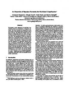
2. Overview of multi-label classification method with LC approach. Figure 2. Figure Overview of multi-label classification method with LC approach. Multi-label Classification Methods

𝒏𝒏

𝟏𝟏 Another approach for this study was the multi-label classification approach. The example of an

∶= ∑ 𝐼𝐼 (𝑌𝑌𝑖𝑖 = 𝑍𝑍𝑖𝑖 ) Multi-label Classification Methods 𝒏𝒏 instance is associated with a set of labels

𝒊𝒊=𝟏𝟏 .

ℒ, |ℒ| > 2

The Label Combination (LC) approach

Another approach ℒ, |ℒ|for > 2this study was the multi-label classification approach. categorized under the PT method isis one of the fundamental of the transformation The example of an instance associated with a problems set of labels 𝑌𝑌 ⊆ ℒ. The 𝒏𝒏 Label Combination (LC) approach categorized under the PT method | |𝑌𝑌 𝟏𝟏 ∩ 𝑍𝑍 𝑖𝑖 method. Figure 2 indicates the methodology of the LC𝑖𝑖 approach adopted in this study. The pre- is ∶= of∑ one of the fundamental problems the transformation method. Figure 2 |𝑌𝑌𝑖𝑖 ∪ 𝑍𝑍𝑖𝑖 | 𝑌𝑌has⊆been ℒ defined in previous𝒏𝒏sections 𝒊𝒊=𝟏𝟏 processingthe stage (Figure 1). In Figure 2, the LC transforms indicates methodology of the LC approach adopted in this study. The pre2ℒ processing has defined(multi-class) in previous sections Figure a multi-labelstage problem intobeen a single-label problem with (Figure possible 1). classIn value by 2, the LC transforms a multi-label problem into a single-label (multi-class) problem with 2ℒ possible class value by treating all label combinations as treating all label combinations as atomic labels, i.e. each label set becomes a single multi-class (𝒙𝒙𝑖𝑖, 𝒀𝒀𝑖𝑖), atomic labels, i.e. each label set becomes a single multi-class label within1 ≤ 𝑖𝑖 ≤ 𝑛𝑛, (𝑥𝑥𝑖𝑖 ∈ label within a single label problem. Consequently, there only 24 24 different classes in thein a single label problem. Consequently, there areareonly different classes thementioned mentioned some activities do innot occur real 𝑘𝑘 datasetsdatasets since somesince activities do not actually occur real actually life. For example, 3in labels 𝑌𝑌𝑖𝑖 ∈ Υ = {0,1} ), |ℒ|distinct ℒ, all = 𝑘𝑘. d, e and f are combined to form def. Thus, the set of single class labels represents 218

13

(𝒙𝒙𝑖𝑖, 𝒀𝒀𝑖𝑖),

ℒ, |ℒ| = 𝑘𝑘.

1 ≤ 𝑖𝑖 ≤ 𝑛𝑛, (𝑥𝑥𝑖𝑖 ∈ 𝑋𝑋,


life. For example, 3 labels d, e and f are combined to form def. Thus, the set of single class labels represents all distinct label subsets in the original multi-label representation. It is also called the distinct labelset, the number of combinations observed in the dataset. Given a new instance, the single-label classifier of LC outputs the most probable class, which is actually a set of labels. If this classifier outputs a probability distribution over all classes, then LC ranks the labels. To obtain a label ranking, it calculates for each label the sum of the probabilities of the classes that contain it. This way LC can solve the complete label correlations task. When the new data arrives, the single label is predicted and then transformed into multi-label vectors for multilabel evaluation and performance assessment. This study experimented with the different base classifiers as mentioned in the previous section in order to evaluate the performance of the proposed method. Validation and Performance Metrics Traditional Multi-class Evaluation Metrics: Validation is required to evaluate the successfulness of classifiers that are able to generalize the solution for new data. This process is necessary to determine how successfully the classifier model learns the characteristics and recognizes the incoming unseen data. K-fold cross-validation performance evaluation techniques are employed in both these experiments. In order to evaluate the performance of the result, several performance indicator metrics were measured. Average accuracy and F-measure were used to evaluate the effectiveness of the work of both classification methods. Multi-label Classification Evaluation Metrics: To evaluate the performance of a single label predicted in testing, the results need to be transformed into multi-label vectors in order to record the performance (details in Figure 2). Hence, a differet evaluation assessment with a special approach should be taken for multi-label classification methods. To treat them as a traditional single label might be too strict for this method. The predictions for an instance is a set of labels, hence the prediction can be fully correct, partially correct or fully incorrect. This makes the assessment of the multi-label classification more challenging than the traditional multi-class classification. For this purpose, we chose to measure the proposed study using the quality of the classification based on the example-based category such as accuracy per label, Hamming score, exact match, and accuracy (Madjarov et al., 2012; Zhang & Zhou, 2014). Meanwhile for label-based measures, the evaluation of each label was computed separately and then averaged over all the labels and any known measure used for the evaluation of a binary classifier (e.g. accuracy, precision, recall, F1, ROC, etc.) can be used here (Sorower, 2010). 219

2ℒ

ℒ, |ℒ| > 2

𝑌𝑌 ⊆ ℒ


2ℒ 𝑌𝑌 ⊆ ℒ

𝑖𝑖

ℒ, |ℒ| = 𝑘𝑘.

𝑖𝑖

(𝒙𝒙𝑖𝑖, 𝒀𝒀𝑖𝑖),

ℒ be a multi-label dataset consisting n multi-label examples Denotion: Let2D (𝒙𝒙𝑖𝑖, ∈ 𝑋𝑋, 𝑌𝑌𝑖𝑖 ∈ Υ = {0,1}𝑘𝑘 ), with a labelset 𝑘𝑘ℒ, |ℒ| = 𝑘𝑘. 𝒀𝒀𝑖𝑖), 1 ≤ 𝑖𝑖 ≤ 𝑛𝑛, (𝑥𝑥𝑖𝑖 (𝒙𝒙𝑖𝑖, 𝑌𝑌𝑖𝑖 𝑘𝑘∈ Υ = {0,1} ), 𝒀𝒀𝑖𝑖), 1 ≤ 𝑖𝑖 𝑛𝑛, (𝑥𝑥𝑖𝑖 ∈ 𝑋𝑋, Let h be a multi-label classifier and≤𝑍𝑍𝑍𝑍 be a set of label = ℎ(𝑥𝑥𝑖𝑖 ) = {0,1} 2ℒ memberships predicted by h for the example of xi. The denotions 𝑘𝑘are applicable (𝒙𝒙𝑖𝑖, 𝒀𝒀𝑖𝑖), 𝑌𝑌𝑖𝑖 ∈ Υ = {0,1} ), 1 ≤ 𝑖𝑖 ≤ 𝑛𝑛, (𝑥𝑥𝑖𝑖 ∈ 𝑋𝑋, for the equations below.

1 ≤ 𝑖𝑖 ≤ 𝑛𝑛, (𝑥𝑥𝑖𝑖

𝑍𝑍𝑍𝑍 = ℎ(𝑥𝑥𝑖𝑖 ) = {0,1}𝑘𝑘 ℒ, |ℒ| = 𝑘𝑘. 𝑛𝑛 ℒ 𝑘𝑘 {0,1} 𝑌𝑌𝑖𝑖 ∈per Υ =label 𝒀𝒀𝑖𝑖), 1 ≤ 𝑖𝑖 ≤ 𝑛𝑛,Score: ), (𝑥𝑥 1 𝑖𝑖 ∈ 𝑋𝑋, Accuracy per (𝒙𝒙𝑖𝑖, label and Hamming Accuracy calculates how ∑ ∑ 𝐼𝐼[𝑍𝑍𝑖𝑖 = 𝑌𝑌𝑖𝑖 ] 𝑛𝑛𝑛𝑛 many times for each the relevance of an example to a class label has ℒ, |ℒ| = label, 𝑘𝑘. 𝑖𝑖=1 𝑖𝑖=1 𝑛𝑛 ℒ 𝑘𝑘 been predicted. 𝑍𝑍𝑍𝑍 = correctly ℎ(𝑥𝑥𝑖𝑖 ) = {0,1} 1 𝑍𝑍𝑍𝑍 = ℎ(𝑥𝑥𝑖𝑖 ) = {0,1}𝑘𝑘 ∑ ∑ 𝐼𝐼[𝑍𝑍𝑖𝑖 = 𝑌𝑌𝑖𝑖 ] ℒ, |ℒ| = 𝑘𝑘. 𝑛𝑛𝑛𝑛

ℒ, |ℒ| = 𝑘𝑘.

𝑖𝑖=1 𝑖𝑖=1 Meanwhile, Hamming score reports the average of the relevance of an example 𝒏𝒏 𝑍𝑍𝑍𝑍 = ℎ(𝑥𝑥𝑖𝑖 ) = {0,1}𝑘𝑘 𝟏𝟏 to a𝑛𝑛class is the indicator function. ℒ label is correctly predicted. Where I(𝑌𝑌 )

∶= ∑ 𝐼𝐼 𝑖𝑖 = 𝑍𝑍𝑖𝑖 1 𝑛𝑛 ℒ 𝒏𝒏 ] 1 ∑ ∑ 𝐼𝐼[𝑍𝑍𝑖𝑖 = 𝑌𝑌 𝑘𝑘 𝒊𝒊=𝟏𝟏 {0,1}= 𝑌𝑌 ] 𝑍𝑍𝑍𝑍 =𝑖𝑖 ℎ(𝑥𝑥 = 𝐼𝐼[𝑍𝑍 𝒏𝒏 𝑛𝑛𝑛𝑛 ∑𝑖𝑖 )∑ Hamming Score: 𝑖𝑖 𝑖𝑖 𝟏𝟏 (1) 𝑖𝑖=1 𝑖𝑖=1 𝑛𝑛𝑛𝑛 𝑛𝑛 𝑖𝑖=1 ℒ 𝑖𝑖=1 ∶= ∑ 𝐼𝐼 (𝑌𝑌𝑖𝑖 = 𝑍𝑍𝑖𝑖 ) 𝒏𝒏 1 𝒊𝒊=𝟏𝟏 ∑ ∑ 𝐼𝐼[𝑍𝑍𝑖𝑖 = 𝑌𝑌𝑖𝑖 ] 𝒏𝒏 𝑛𝑛𝑛𝑛 𝑛𝑛multi-label ℒ 𝟏𝟏 it |𝑌𝑌 ∩ 𝑍𝑍𝑖𝑖 | 𝑖𝑖=1 Exact𝒏𝒏 Match: 1In𝑖𝑖=1 prediction is𝑖𝑖 partially correct to ignore it ∶= ∑ 𝟏𝟏 𝒏𝒏 | |𝑌𝑌 𝒏𝒏 accuracy ∑ ∑ 𝐼𝐼[𝑍𝑍 𝑌𝑌𝑖𝑖 ] (consider it as incorrect) and the in a single label case 𝑖𝑖 ∪ 𝑍𝑍used 𝑖𝑖 𝑖𝑖 = extend ∑ 𝐼𝐼 (𝑌𝑌 ∶= 𝑍𝑍𝑖𝑖 ) 𝟏𝟏 𝒊𝒊=𝟏𝟏 𝑖𝑖 =𝑛𝑛𝑛𝑛 𝒏𝒏 ∶= 𝑖𝑖=1∑ 𝐼𝐼 (𝑌𝑌𝑖𝑖 = 𝑍𝑍𝑖𝑖 ) 𝑖𝑖=1 for𝒏𝒏a𝒊𝒊=𝟏𝟏 multi-label prediction. |𝑌𝑌𝑖𝑖 ∩ 𝑍𝑍𝑖𝑖 | 𝟏𝟏 𝒏𝒏 𝒏𝒏 𝒊𝒊=𝟏𝟏 ∶= ∑ |𝑌𝑌𝑖𝑖 ∪ 𝑍𝑍𝑖𝑖 | 𝒏𝒏 𝟏𝟏 𝒊𝒊=𝟏𝟏 ∑ 𝐼𝐼 (𝑌𝑌𝑖𝑖 = 𝑍𝑍𝑖𝑖 ) Exact Match: ∶= (2) 𝒏𝒏 𝒏𝒏 𝒊𝒊=𝟏𝟏 𝒏𝒏 𝟏𝟏 |𝑌𝑌𝑖𝑖 ∩ 𝑍𝑍 𝟏𝟏 𝑖𝑖 | ∑ 𝐼𝐼 𝒏𝒏 (𝑌𝑌𝑖𝑖|𝑌𝑌= 𝑍𝑍𝑖𝑖 ) | ∶= 𝟏𝟏 ∶= ∑ 𝑖𝑖 ∩ 𝑍𝑍𝑖𝑖 |𝑌𝑌𝑖𝑖 Accuracy ∪ 𝑍𝑍𝑖𝑖 | 𝒏𝒏∶= 𝒏𝒏 ∑ each instance is defined as the proportion of the 𝒊𝒊=𝟏𝟏 for Accuracy: 𝒊𝒊=𝟏𝟏 |𝑌𝑌𝑖𝑖 ∪ 𝑍𝑍𝑖𝑖 | 𝒏𝒏 𝒏𝒏 𝒊𝒊=𝟏𝟏 predicted correct𝟏𝟏labels total number (predicted and actual) of labels for |𝑌𝑌𝑖𝑖to∩the 𝑍𝑍𝑖𝑖 | ∑ accuracy is the average across all instances. that instance. ∶= Overall |𝑌𝑌𝑖𝑖 ∪ 𝑍𝑍𝑖𝑖 | 𝒏𝒏 𝒏𝒏 𝒊𝒊=𝟏𝟏 |𝑌𝑌𝑖𝑖 ∩ 𝑍𝑍𝑖𝑖 | 𝟏𝟏 Accuracy (A):∶= (3) ∑ |𝑌𝑌𝑖𝑖 ∪ 𝑍𝑍𝑖𝑖 | 𝒏𝒏 𝒊𝒊=𝟏𝟏

EXPERIMENTAL RESULTS AND DISCUSSIONS As mentioned previously, the purpose of this work was to evaluate the performance of the proposed classifier model to recognize various kinds of human activities with the efficient placement of the sensor. In this experiment, two different sets of experiments were done to compare the performance between the traditional multi-class and the multi-label classification methods. Both experiments were conducted using the 10-fold cross validation technique. Four different types of classifiers, namely rotation forest, SVM, J48 and MLP were utilized. In the traditional multi-class classification approach, the rotation forest, decision tree J48 classifier model was used as a base classifier and PCA 220


was used to generate the feature subsets. Default parameter values were used for the rest of the classifier models: SVM, J48 and MLP. The initial steps were performed using the same parameter setting, including pre-processing and feature extraction. Experiment 1: Traditional Multi-class Classification Approach This subsection explains the experiment using the traditional multi-class classification approach. The initial steps were performed using the same parameter setting, including the pre-processing and feature extraction stages. However, the representatives of the class labeling were different for both experiments. Only one label was required for the traditional multi-class classification approach representing the class of activity performed. Each dataset from each sensor position represented one class label. Hence, the experiment was conducted in four separate datasets. Table 2 (a) - (d) indicate the classification result using several classification methods for each sensor placement; arm, belt, pocket and wrist respectively. Table 2(a) Classification Result of Arm Sensor Placement Rotation forest Activity

SVM

J48

MLP

Accuracy

F-measure

Accuracy

F-measure

Accuracy

F-measure

Accuracy

Downstairs

0.961

0.963

0.126

0.208

0.924

0.933

0.470

0.543

Upstairs

0.929

0.945

0.386

0.513

0.923

0.913

0.666

0.703

Walking

0.995

0.984

0.326

0.415

0.962

0.960

0.733

0.686

Running

0.999

0.998

0.990

0.804

0.992

0.992

0.982

0.983

Sitting

1.000

0.999

0.607

0.613

0.981

0.981

0.872

0.799

Standing

0.998

0.999

0.484

0.527

0.974

0.977

0.657

0.685

Average

0.989

0.989

0.653

0.613

0.972

0.972

0.819

0.816

Time

6.25

11.94

F-measure

0.27

49.74

J48

MLP

Table 2(b) Classification Result of Belt Sensor Placement Rotation forest Activity

Downstairs

Accuracy 0.935

F-measure 0.941

SVM Accuracy 0.438

F-measure 0.548

Accuracy

F-measure

0.925

0.916

Accuracy 0.703

F-measure 0.748

(continued) 221


Rotation forest Activity

Accuracy

F-measure

SVM Accuracy

J48

F-measure

MLP

Accuracy

F-measure

Accuracy

F-measure

Upstairs

0.953

0.951

0.410

0.547

0.913

0.914

0.765

0.784

Walking

0.992

0.992

0.421

0.489

0.961

0.963

0.721

0.698

Running

0.988

0.986

0.673

0.610

0.965

0.969

0.880

0.880

Sitting

0.996

0.997

0.753

0.516

0.984

0.984

0.824

0.800

Standing

1.000

1.000

0.716

0.798

0.981

0.981

0.943

0.953

Average

0.982

0.982

0.583

0.588

0.959

0.959

0.814

Time

4.05

5.53

0.3

0.815 34.83

Table 2(c) Classification Result of Pocket Sensor Placement Rotation forest Activity

SVM

Accuracy

F-measure

Downstairs

0.954

0.959

0.093

Upstairs

0.969

0.974

0.457

Walking

0.988

0.981

Running

0.988

0.989

Sitting

1.000

Standing

1.000

Average

0.986

Time

Accuracy

J48 Accuracy

F-measure

0.158

0.901

0.886

0.515

0.549

0.502

0.909

0.913

0.660

0.654

0.743

0.464

0.926

0.929

0.680

0.705

0.597

0.592

0.959

0.959

0.843

0.819

1.000

0.509

0.600

0.992

0.994

0.852

0.806

1.000

0.593

0.701

0.994

0.995

0.880

0.894

0.986

0.530

0.526

0.951

0.951

0.756

0.754

4.15

F-measure

MLP

5.64

Accuracy

0.33

F-measure

34.38

Table 2(d) Classification Result of Wrist Sensor Placement Rotation forest Activity

Accuracy

F-measure

SVM Accuracy

J48

F-measure

Accuracy

MLP F-measure

Accuracy

F-measure

Downstairs

0.973

0.976

0.118

0.195

0.918

0.910

0.450

0.559

Upstairs

0.956

0.967

0.577

0.722

0.897

0.907

0.727

0.760

Walking

0.990

0.980

0.744

0.560

0.956

0.950

0.864

0.758

Running

1.000

1.000

0.603

0.702

0.986

0.986

0.930

0.900

Sitting

1.000

0.999

0.616

0.741

0.984

0.985

0.879

0.876

Standing

0.995

0.996

0.849

0.631

0.975

0.977

0.843

0.871

Average

0.988

0.988

0.621

0.613

0.958

0.958

0.809

0.804

Time

4.04

5.39

0.2

222

33.7


The classification result obtained for each sensor position was led by the rotation forest classifier model where the average accuracy and F-measure recorded was above 98%. Stationary activities such as sitting recorded 100% accuracy for each placement; arm, pocket and wrist. Two-stairs activities (downstairs and upstairs) reported a slightly lower accuracy than the other since both of these activities always confuse each other because the signal produced from both the activities are very similar. J48 recorded the second highest methods that brought out a beneficial resolution to recognize the types of activity performed. The optimized result obtained from this method was recorded from an arm placement where the accuracy and F-measure obtained 97%. The best sensor placement recorded by MLP was from the arm, then the belt followed by the wrist since above 80% accuracy was recorded for accuracy and F-measure. However, pocket placement recorded the lowest result, below 76% accuracy using MLP. Two placements which recorded the best from SVM (arm and wrist) were above 62% accuracy as reported in Table 2 followed by the belt and the wrist placements. To tackle the best time taken to build the classifier model chosen, the total time taken to develop the classifier model is as tabulated in Table 3. Table 3 Overall Time (in Seconds) Consumed for Each Classifier Model Classifier model / Position

Rotation forest

SVM

J48

MLP

Arm

6.25

11.94

0.27

49.74

Belt

4.05

5.53

0.3

34.83

Pocket

4.15

5.64

0.33

34.38

Wrist

4.04

5.39

0.2

33.7

1.1

152.65

Total (in seconds)

18.49

28.5

It is clear that MLP recorded the longest time required to build the training model. A total of 152.65 seconds was consumed for each of the sensor placements; arm, belt, pocket and wrist. Even though the average accuracy recorded from the MLP was better than SVM, the time required to build the training model was five times longer than SVM. J48 recorded the shortest time taken for all sensor placements which was less than 0.4 seconds required for the classifier model. Meanwhile, the average accuracy recorded by rotation forest outperformed other classifier models, but the time required for the training model was somewhat longer than J48. This was caused because this 223


ensemble classifier model required more sets of trees to create the classifier model compared to the traditional decision-tree classifier model. Experiment 2: Multi-label Classification Methods This experiment was implemented using a single dataset combination from four different files of the arm, belt, pocket and wrist activity types. Its labelset consisted of 10 labels with details of the types of activity and sensor placements represented respectively (6 types of activity and 4 different sensor placements). Table 4 shows the result of per label accuracy of the LC approach under different base classifiers. LC with rotation forest was the most accurate for every label compared to other base classifiers. It recorded 99% accuracy for downstairs, sitting and standing activities and sensor placement belt. Other than that, activities like running and walking were 99.7% and 99.2% accurate respectively. Sensor placements at arm, pocket and wrist were 99.8% and 97.7% accurate respectively. However, upstairs recorded 98.8% the least. This shows that the sensor placement at the belt is the most suitable place for downstairs, sitting and standing (99.9%) activities followed by running and walking (99.7% and 99.2%) and lastly upstairs (98.8%). Table 4 Accuracy Per Label of LC Approach Using a Different Base Classifier Base Classifier / Activity & Sensor Placement

Accuracy per label

Rotation Forest

J48

SVM

MLP

Downstairs

0.99

0.976

0.904

0.901

Running

0.997

0.986

0.819

0.918

Sitting

0.999

0.993

0.838

0.885

Standing

0.999

0.99

0.772

0.898

Upstairs

0.988

0.972

0.883

0.869

Walking

0.992

0.978

0.811

0.833

Arm

0.998

0.983

0.725

0.858

Belt

0.999

0.991

0.788

0.874

Pocket

0.997

0.984

0.858

0.882

Wrist

0.997

0.982

0.777

0.858

The overall performance of LC is reported in Table 5 with the time taken to build the activity model. Hamming scores of rotation forest show 99.6%, 224


the best compared to other classifiers; 98.3% for J48, 0.878 for MLP and 81.7% for SVM, the smallest value. Hence, accuracy and exact match of rotation forest also recorded the most significant results compared to other base classifiers with 98.9% and 98.1% respectively followed by J48, MLP and SVM. However the average precision of SVM with 46.2% was the highest. Similarly, with the traditional multi-class method, MLP also recorded the longest time with 306.208 seconds required to build the training model for the activities and sensor placements. Rotation forest required 34.441 seconds to build its model. Even though the hamming score recorded by rotation forest was the higher than J48 and SVM, the time required to build the training model for J48 was the shortest with only 2.334 seconds and SVM with 26.125 seconds. To summarize, similar to the traditional multi-class model, the overall performance of the LC approach with rotation forest excelled compared to the other base classifiers. Nevertheless, the time required for the training model was 32.107 seconds longer than J48. Table 5 Overall Performance Of LC Method Time Taken to Build The Classifier Model Rotation forest

J48

SVM

MLP

Hamming score

0.996

0.983

0.817

0.878

Accuracy

0.989

0.961

0.615

0.734

Exact match

0.981

0.937

0.418

0.591

F1 (micro averaged)

0.993

0.974

0.709

0.805

F1 (macro averaged by label)

0.99

0.962

0.58

0.718

34.441

2.334

26.125

306.208

Base classifier

Total build time (in sec)

CONCLUSION This study reported the effectiveness of the traditional multi-class and the multilabel classification methods to undertake the problem of finding an optimal sensor placement with the activity performed. In this study, a public domain activity dataset consisting of six different types of stationary and locomotion activities was experimented upon. The acceleration signal underwent a filtering process to remove unwanted information. A Butterworth low pass filter was applied to separate the acceleration signal between two signal notations; body 225


acceleration and gravitational acceleration. In order to segment the signal into a series of smaller window segments, a sliding window with 50% overlapping between two adjacent window segments was used. Additional features from statistical descriptors and spectral analysis were employed to provide more information for the classifier model to learn the characteristics of each class. Two classification approaches were proposed; the traditional approach and the multi-label approach. Rotation forest, SVM, J48 and MLP were utilized and compared with the former ones. Next, the same classifiers were also used as base classifiers in the second approach. Rotation forest achieved the best accuracy in recognizing the various types of activities for each sensor placement. In terms of time consuming, treebased classifier J48 outperformed other classifier models. However, it became problematic to conduct the same experiment setting of each sensor placement using traditional approaches. Hence, in order to increase the efficiency of the recognition process, the multi-label classification approach was introduced to recognize the activities with several numbers of labels. Thus, this approach took place to classify several types of classes such as the activity class and sensor placements in one whole subset. Consequently, the multilabel classification approach showed 99.6% accuracy. The Hamming score using the rotation forest indicated the most excellent result compared with the traditional multi-class classification approach. Thus, in the multi-label classification approach, the belt position showed the most suitable position to perform the six activities at the same time. Meanwhile, using the traditional multi-class classification approach, the arm showed the most excellent result to perform the six activities at the same time. Still, the multi-label classification approach produced the most excellent result between both approaches. Hence, this approach eliminated the manual work for generating the model as well as to improving the accuracy for recognizing the activities being performed. For future work, we plan to investigate the proposed method in another domain area such as text mining and the user profiling in a smart home. REFERENCES Abidine, M. B., & Fergani, B. (2012). Evaluating C -SVM , CRF and LDA classification for daily activity recognition. Paper presented in the Conference on Multimedia Computing and System (ICMCS), 272-277. Doi: 10.1109/ICMCS.2012.6320300 Acharjee, D., Mukherjee, A., Mandal, J. K., & Mukherjee, N. (2015). Activity recognition system using inbuilt sensors of smart mobile phone and minimizing feature vectors. Microsystem Technologies. http://doi. org/10.1007/s00542-015-2551-2 226


Alsheikh, M. A., Selim, A., Niyato, D., Doyle, L., Lin, S., & Tan, H.-P. (2015). Deep activity recognition models with triaxial accelerometers. In The Workshops of the Thirtieth AAAI Conference on Artificial Intelligence (pp. 1–8). Anguita, D., Ghio, A., Oneto, L., Parra, X., & Reyes-Ortiz, J. L. (2013). A public domain dataset for human activity recognition using smartphones. European Symposium on Artificial Neural Networks, Computational Intelligence and Machine Learning, (April), 24–26. Antos, S. A., Albert, M. V., & Kording, K. P. (2014). Hand, belt, pocket or bag: Practical activity tracking with mobile phones. Journal of Neuroscience Methods, 231, 22–30. http://doi.org/10.1016/j.jneumeth.2013.09.015 Arif, M., Bilal, M., & Kattan, A. (2014). Better physical activity classification using smartphone acceleration sensor. Retrieved from http://doi. org/10.1007/s10916-014-0095-0 Arif, M., & Kattan, A. (2015). Physical activities monitoring using wearable acceleration sensors attached to the body. PLoS ONE, 10(7), 1–16. http://doi.org/10.1371/journal.pone.0130851 Banos, O., Galvez, J., Damas, M., Pomares, H., & Rojas, I. (2014). Window size impact in human activity recognition, 6474–6499. http://doi. org/10.3390/s140406474 Bao, L., & Intille, S. S. (2004). Activity recognition from user-annotated acceleration data. Pervasive Computing, 1–17. http://doi.org/10.1007/ b96922 Blockeel, H., Schietgat, L., Struyf, J., & Clare, A. (2008). Decision trees for hierarchical multilabel classification : A case study in functional genomics. Brezovan, M., & Badica, C. (2013). A review on vision surveillance techniques in smart home environments. Proceedings - 19th International Conference on Control Systems and Computer Science, CSCS 2013, 471–478. http://doi.org/10.1109/CSCS.2013.30 Catal, C., Tufekci, S., Pirmit, E., & Kocabag, G. (2015). On the use of ensemble of classifiers for accelerometer-based activity recognition. Applied Soft Computing Journal, 1–5. http://doi.org/10.1016/j.asoc.2015.01.025 227


Fang, H., He, L., Si, H., Liu, P., & Xie, X. (2014). Human activity recognition based on feature selection in smart home using back-propagation algorithm. ISA Trans, 53, 1629–1638. Fleury, A., Vacher, M., & Noury, N. (2010). SVM-based multimodal classification of activities of daily living in health smart homes: Sensors, algorithms, and first experimental results. IEEE Transactions on Information Technology in Biomedicine, 14(2), 274–283. http://doi. org/10.1109/TITB.2009.2037317 Foerster, F., Smeja, M., & Fahrenberg, J. (1999). Detection of posture and motion by accelerometry: A validation study in ambulatory monitoring. Computers in Human Behavior, 15(5), 571–583. http://doi.org/10.1016/ S0747-5632(99)00037-0 Goh, K. L., Member, I., Lim, K. H., Member, I., Gopalai, A. A., Member, I., & Chong, Y. Z. (2014). Multilayer perceptron neural network classification for human vertical ground reaction forces, (December), 8–10. Guiry, J. J., van de Ven, P., Nelson, J., Warmerdam, L., & Riper, H. (2014). Activity recognition with smartphone support. Medical Engineering and Physics, 36, 670–675. http://doi.org/10.1016/j.medengphy.2014.02.009 Hasrul Mohd Nazid, Hariharan Muthusamy, Vikneswaran Vijean, S. Y. (2015). Improved speaker-independent emotion recognition from speech using two-stage feature reduction. Journal of ICT, 14, 57–76. Retrieved from http://www.jict.uum.edu.my/images/pdf/vol14/jict144.pdf Kwapisz, J. R., Weiss, G. M., & Moore, S. a. (2011). Activity recognition using cell phone accelerometers. ACM SIGKDD Explorations Newsletter, 12, 74. http://doi.org/10.1145/1964897.1964918 Lara, O. D., & Labrador, M. a. (2012). A survey on human activity recognition using wearable sensors. IEEE Communications Surveys & Tutorials, 1–18. http://doi.org/10.1109/SURV.2012.110112.00192 M.a, A., A.a, K., & S.I.b, A. (2015). Classification of physical activities using wearable sensors. Intelligent Automation and Soft Computing, (September 2016), 1–10. http://doi.org/10.1080/10798587.2015.11182 75 Machado, I. P., Luisa Gomes, A., Gamboa, H., Paixao, V., & Costa, R. M. (2015). Human activity data discovery from triaxial accelerometer 228


sensor: Non-supervised learning sensitivity to feature extraction parametrization. Information Processing and Management, 51(2), 201– 214. http://doi.org/10.1016/j.ipm.2014.07.008 Madjarov, G., Kocev, D., Gjorgjevikj, D., & Dzeroski, S. (2012). An extensive experimental comparison of methods for multi-label learning. Pattern Recognition, 45(9), 3084–3104. http://doi.org/10.1016/j. patcog.2012.03.004 Mannini, A., Intille, S. S., Rosenberger, M., Sabatini, A. M., & Haskell, W. (2013). Activity recognition using a single accelerometer placed at the wrist or ankle. Medicine and Science in Sports and Exercise, 45(11). http://doi.org/10.1249/MSS.0b013e31829736d6 Mannini, A., Sabatini, A. M., & Intille, S. S. (2015). Accelerometry-based recognition of the placement sites of a wearable sensor. Pervasive and Mobile Computing, 21, 62–74. http://doi.org/10.1016/j. pmcj.2015.06.003 Miyamoto, S., & Ogawa, H. (2014). Human activity recognition system including smartphone position. Procedia Technology, 18(September), 42–46. http://doi.org/10.1016/j.protcy.2014.11.010 Mohamed, R., Perumal, T., Sulaiman, M. N., & Mustapha, N. (2017). Multiresident complex activity recognition in smart home : A literature review. International Journal of Smart Home, Vol. 11(No. 6 (2017)), 21–32. Retrieved from http://www.sersc.org/journals/IJSH/vol11_ no6_2017.php Mohamed, R., Perumal, T., Sulaiman, M. N., Mustapha, N., & Zainudin, M. N. S. (2016). Multi label classification on multi resident in smart home using classifier chains, 8–12. http://doi.org/10.1166/asl.2011.1261 Noury, N., & Hadidi, T. (2012). Computer simulation of the activity of the elderly person living independently in a health smart home. Computer Methods and Programs in Biomedicine, 108, 1216–1228. http://doi. org/10.1016/j.cmpb.2012.07.004 Qian, H., Mao, Y., Xiang, W., & Wang, Z. (2010). Recognition of human activities using SVM multi-class classifier. Pattern Recognition Letters, 31(2), 100–111. http://doi.org/10.1016/j.patrec.2009.09.019 Quinlan, J. R. (1986). Induction of decision trees. Machine Learning, 1(1), 81–106. http://doi.org/10.1023/A:1022643204877 229


Rahim, R. A., Othman, N., Zainudin, M. N. S., Ali, N. A., & Ismail, M. M. (2012). Iris recognition using histogram analysis via LPQ and RI-LPQ Method, (4), 66–70. Read, J., & Hollmen, J. (2014). A deep interpretation of classifier chains. In Advances In Intelligent Data Analysis XIII (Vol. 8819, pp. 251–262). Reyes Ortiz, J. L. (2015). Smartphone-based human activity recognition, (2012). http://doi.org/10.1007/978-3-319-14274-6 Rodríguez, J. J., Kuncheva, L. I., & Alonso, C. J. (2006). Rotation forest: A new classifier ensemble method. IEEE Transactions on Pattern Analysis and Machine Intelligence, 28(10), 1619–1630. http://doi.org/10.1109/ TPAMI.2006.211 Schapire, R. E., & Singer, Y. (2000). BoosTexter: A boosting- based system for text categorization. Machine Learning, 39, 135–168. Retrieved from http://link.springer.com/article/10.1023/A:1007649029923 Shoaib, M., Bosch, S., Durmaz Incel, O., Scholten, H., & Havinga, P. J. M. (2014). Fusion of smartphone motion sensors for physical activity recognition. Sensors (Switzerland) (Vol. 14). http://doi.org/10.3390/ s140610146 Shoaib, M., Scholten, H., & Havinga, P. J. M. (2013). Towards physical activity recognition using smartphone sensors. 2013 IEEE 10th International Conference on Ubiquitous Intelligence and Computing and 2013 IEEE 10th International Conference on Autonomic and Trusted Computing, 80–87. http://doi.org/10.1109/UIC-ATC.2013.43 Sorower, M. S. (2010). A literature survey on algorithms for multi-label learning. Technical report. USA: Oregon State University, Corvallis, Oregon (December). Struyf, J., Džeroski, S., Blockeel, H., & Clare, A. (2005). Hierarchical multiclassification with predictive clustering trees in functional genomics. In Lecture Notes in Computer Science (including subseries Lecture Notes in Artificial Intelligence and Lecture Notes in Bioinformatics) (Vol. 3808 LNCS, pp. 272–283). http://doi.org/10.1007/11595014_27 Su, X., Tong, H., & Ji, P. (2014). Activity recognition with smartphone sensors. Tsinghua Science and Technology, 19(3), 235–249. http://doi.org/10.1109/ TST.2014.6838194 230


Sun, L., Zhang, D., Li, B., Guo, B., & Li, S. (2010). Activity recognition on an accelerometer embedded mobile phone with varying positions and orientations, 548–562. Tiong, L., Ow, C., Chek, D., Ngo, L., & Lee, Y. (2016). Prediction of forex trend movement using linear regression line, two-stage of multi-layer perceptron and dynamic time warping algorithms. Journal of ICT, 15(2), 117–140. Retrieved from http://www.jict.uum.edu.my/images/ pdf3/vol15no2/6jictno22016.pdf Tsoumakas, G., & Katakis, I. (2007). Multi-label classification: An overview. In Database Technologies (Vol. 3, pp. 309–319). IGI Global. http://doi. org/10.4018/978-1-60566-058-5.ch021 Tsoumakas, G., Katakis, I., & Vlahanas, I. (2010). Mining multi-label data. Data Mining and Knowledge Discovery Handbook, (Mlc), 667–685. http://doi.org/10.1088/1751-8113/44/8/085201 Walse, K. H., Dharaskar, R. V, & Thakare, V. M. (2016). A study of human activity recognition using adaboost classifiers on wisdm dataset. Iioab Journal, 7(2, SI), 68–76. WHO. (2016). WHO. World Health Day 2016: WHO calls for global action to halt rise in and improve care for people with diabetes. Retrieved April 6, from https://ncdalliance.org/news-events/news/world-healthy-day-2016 Wu, W., Dasgupta, S., Ramirez, E. E., Peterson, C., & Norman, G. J. (2012). Classification accuracies of physical activities using smartphone motion sensors. Journal of Medical Internet Research, 14(5), 1–9. http://doi. org/10.2196/jmir.2208 Zainudin, M. N. S., Radi, H. ., & Abdullah, S. (2012). Face recognition using principle component analysis (PCA) and linear discriminant analysis (LDA). Ijens.Org, (5). Zainudin, M. N. S., Sulaiman, N., Mustapha, N., & Perumal, T. (2015). Activity recognition based on accelerometer sensor using combinational classifiers (pp. 68–73). Zhang, M., & Zhou, Z. (2014). A review on multi-label learning algorithms. IEEE Transactions on Knowledge and, 26(8), 1819–1837. Retrieved from http://ieeexplore.ieee.org/xpls/abs_all.jsp?arnumber=6471714 231