An Ensemble of Bayesian Networks for Multilabel Classification∗ Antonucci Alessandro? , Giorgio Corani? , Denis Mau´a? , and Sandra Gabaglio† ? Istituto “Dalle Molle” di Studi sull’Intelligenza Artificiale (IDSIA), Manno (Switzerland) {alessandro,giorgio,denis}@idsia.ch † Istituto Sistemi Informativi e Networking (ISIN), Manno (Switzerland)
[email protected] Abstract We present a novel approach for multilabel classification based on an ensemble of Bayesian networks. The class variables are connected by a tree; each model of the ensemble uses a different class as root of the tree. We assume the features to be conditionally independent given the classes, thus generalizing the naive Bayes assumption to the multiclass case. This assumption allows us to optimally identify the correlations between classes and features; such correlations are moreover shared across all models of the ensemble. Inferences are drawn from the ensemble via logarithmic opinion pooling. To minimize Hamming loss, we compute the marginal probability of the classes by running standard inference on each Bayesian network in the ensemble, and then pooling the inferences. To instead minimize the subset 0/1 loss, we pool the joint distributions of each model and cast the problem as a MAP inference in the corresponding graphical model. Experiments show that the approach is competitive with state-of-the-art methods for multilabel classification.
1
Introduction
In traditional classification each instance belongs only to a single class. Multilabel classification generalizes this idea by allowing each instance to belong to different relevant classes at the same time. A simple approach to deal with multilabel classification is binary relevance (BR): a binary classifier is independently trained for each class and then predicts whether such class is relevant or not for each instance. BR ignores dependencies among the different classes; yet it can be quite competitive [Dembczynski et al., 2012] especially under loss functions which decompose label-wise, such as the Hamming loss. Instead the global accuracy (also called exact match) does not decompose label-wise; a classification is regarded as accurate only if the relevance of every class has been correctly ∗ Work supported by the Swiss NSF grant no. 200020 134759 / 1 and by the Hasler foundation grant n. 10030.
identified. To obtain good performance under global accuracy, it is necessary identifying the maximum a posteriori (MAP) configuration, that is, the mode of the joint probability distribution of the classes given the features, which in turn requires to properly model the stochastic dependencies among the different classes. A state-of-the-art approach to this end is the classifier chain (CC) [Read et al., 2011]. Although CC has not been designed to minimize a specific loss function, it has been recently pointed out [Dembczynski et al., 2010; 2012] that it can be interpreted as a greedy approach for identifying the mode of the joint distribution of the classes given the value of the features; this might explain its good performance under global accuracy. Bayesian networks (BNs) are a powerful tool to learn and perform inference on the joint distribution of several variables; yet, they are not commonly used in multilabel classification. They pose two main problems when dealing with multilabel classification: learning from data the structure of the BN model and performing inference on the learned model in order to issue a classification. In [Bielza et al., 2011], the structural learning problem is addressed by partitioning the arcs of the structure into three sets: links among the class variables (class graph), links among features (features graph) and links between class and features variables (bridge graph). Each subgraph is separately learned and can have different topology (tree, polytree, etc). Inference is performed either by an optimized enumerative scheme or by a greedy search, depending on the number of classes. Thoroughly searching for the best structure introduces the issue of model uncertainty: several structures, among the many analyzed, might achieve similar scores and thus the model selection can become too sensitive on the specificities of the training data, eventually increasing the variance component of the error. In traditional classification, this problem has been successfully addressed by instantiating all the BN classifiers whose structure satisfy some constraints and then combining their inferences, avoiding thus an exhaustive search for the best structure [Webb et al., 2005]. The resulting algorithm, called AODE, is indeed known to be a highperformance classifier. In this paper, we extend to the multilabel case the idea of averaging over a constrained family of classifiers. We assume the graph connecting the classes to be a tree. Rather than searching for the optimal tree, we instantiate a differ-
ent classifier for each class; each classifier adopts a different class as root. We moreover assume the independence of the features given the classes, thus generalizing to the multilabel case the naive Bayes assumption. This implies that the subgraph connecting the features is empty. Thanks to the naivemultilabel assumption, we can identify the optimal subgraph linking classes and the features in polynomial time [de Campos and Ji, 2011]. This optimal subgraph is the same for all the models of the ensemble, which speeds up inference and learning. Summing up: we perform no search for the class graph, as we take the ensemble approach; we perform no search for the feature graph; we perform an optimal search for the bridge graph. Eventually, we combine the inferences produced by the members of the ensemble via geometric average (logarithmic opinion pool), which minimizes the average KL-divergence between the true distribution and the elements of an ensemble of probabilistic models [Heskes, 1997]. It is moreover well known that simple combination schemes (such as arithmetic average or geometric average) often dominates more refined combination schemes [Yang et al., 2007; Timmermann, 2006]. The inferences are tailored to the loss function being used. To minimize Hamming loss, we query each classifier of the ensemble about the posterior marginal distribution of each class variable, and then pool such marginals to obtain an ensemble probability of each class being relevant. To instead maximize the global accuracy, we compute the MAP inference in the pooled model. Although both the marginal and joint inferences are NP-hard in general, they can often be performed quite efficiently by state-of-the-art algorithms.
2
Probabilistic Multilabel Classification
We denote the array of class events as C = (C1 , . . . , Cn ); this is an array of Boolean variables which expresses whether each class label is relevant or not for the given instance. Thus, C takes its values in {0, 1}n . A instantiation of class events is denoted as c = (c1 , . . . , cn ). We denote the set of features as F = (F1 , . . . , Fm ). An instantiation of the features is denoted as f = (f1 , . . . , fm ). A set of complete training instances D = {(c, f )} is supposed to be available. ˆ and ˜ For a generic instance, we denote as c c respectively the labels assigned by the classifier and the actual labels; similarly, with reference to class ci , we denote as cˆi and c˜∗i its predicted and actual labels. The most common metrics to evaluate multilabel classifiers are the global accuracy (a.k.a. exact match), denoted as acc, and the Hamming loss (HL). Rather than HL, we use in the following the Hamming accuracy, defined as Hacc =1-HL. This simplifies the interpretation of the results as both acc and Hacc are better when they are higher. The metrics are defined as follows: n X acc = δ(ˆ c, ˜ c ), Hacc = n−1 δ(ˆ ci , c˜i ). i=1
A probabilistic multilabel classifier classifies data according to a conditional joint probability distribution P (C|F). Our approach consists in learning an ensemble of probabilistic classifiers that jointly approximate the (unknown) true distribution P (C|F). When classifying an instance with features
f , two different kinds of inference are performed depending on whether the goal is maximizing global accuracy or Hamˆ maximizes ming accuracy. The most probable joint class c global accuracy (under the assumption that P (C|F) is the true distribution), and is given by ˆ = arg max P (c|f ). c n c∈{0,1}
(1)
The maximizer of Hamming accuracy instead consists in selecting the most probable marginal class label separately for each Ci ∈ C: cˆi = arg max P (ci |f ), ci ∈{0,1}
(2)
P with P (ci |f ) = C\{Ci } P (c|f ). The choice of the appropriate inference to be performed given a specific loss function is further discussed in [Dembczynski et al., 2012].
3
An Ensemble of Bayesian Classifiers
As with traditional classification problems, building a multilabel classifier involves a learning phase, where the training data are used to tune parameters and perform model selection, and a test phase, where the learned model (or in our case, the ensemble of models) is used to classify instances. Our approach consists in learning an ensemble of Bayesian networks from data, and then merging these models via geometric average (logarithmic pooling) to produce classifications. Bayesian networks [Koller and Friedman, 2009] provide a compact specification for the joint probability mass function of class and feature variables. Our ensemble contains n different Bayesian networks, one for each class event Ci (i = 1, . . . , n), each providing an alternative model of the joint distribution P (C, F).
3.1
Learning
The networks in the ensemble are indexed by the class events. With no lack of generality, we describe here the network associated to class Ci . First, a directed acyclic graph Gi over C such that Ci is the unique parent of all the other class events, and no more arcs are present, is considered (see Fig. 1.a). Following the Markov condition,1 this corresponds to assume that, given Ci , the other classes are independent. The features are assumed to be independent given the joint class C. This extends the naive Bayes assumption to the multilabel case. At the graph level, the assumption can be accomodated by augmenting the graph Gi , defined over C, to a graph G i defined over the whole set of variables (C, F) as follows. The features are leaf nodes (i.e., they have no children) and their parents are, for each feature, all the class events (see Fig. 1.b). A Bayesian network associated to G i has maximum indegree (i.e., maximum number of parents) equal to the number of classes n: there are therefore conditional probability tables whose number of elements is exponential in n. This is not practical for problems with many classes. A structural learning algorithm can be therefore adopted to reduce 1
The Markov condition for directed graphs specifies the graph semantics in Bayesian networks: any variable is conditionally independent of its non-descendant non-parents given its parents.
the maximum in-degree. In practice, to remove some classto-feature arcs in G i , we evaluate the output of the following optimization: Gi∗ = arg max log P (G|D),
with the values of fj , ci , cl , cFj consistent with those of c, f . Note that according to the above model assumptions, the data likelihood term
(3)
Gi ⊂G⊂G i
where set inclusions among graphs should be intended in the arcs space, and log P (G|D) =
n X
ψα [Ci , Pa(Ci )] +
i=1
m X
where the second sum is over the possible states of Fj , and the first over the joint states of its parents. Moreover, Njik is the number of records such that Fj is in its k-thP state and its parents in their i-th configuration, while Nji = k Njik . Finally, αji is equal to α divided by the number of states of Fj and by the P number of (joint) states of the parents of Fj , while αj = i αji . If we consider a network associated to a specific class event, the links connecting the class events are fixed; thus, the class variables have the same parents for all the graphs in the search space. This implies that the first sum in the right-hand side of (4) is constant. The optimization in (3) can be therefore achieved by considering only the features. Any subset of C is a candidate for the parents set of a feature, this reducing the problem to m independent local optimizations. In practice, the parents of Fj according to G ∗ are ψα [Fj , Pa(Fj )],
Y l=1,...,n,l6=i
P (cl |ci ) ·
C2
C2
(a) Graph G1 (n = 3).
j=1
F2
(b) Augmenting G1 to G 1 (m = 2).
C1
C2
F1
C3
F2
(c) Removing class-to-feature arcs from G 1 to obtain G1∗ .
Figure 1: The construction of the graphs of the Bayesian networks in the ensemble. The step from (b) to (c) is based on the structural learning algorithm in (6).
3.2
m Y
F1
C3
C3
(6)
for each j = 1, . . . , m. This is possible because of the bipartite separation between class events and features, while in general cases the graph maximizing all the local scores can include directed cycles. Moreover, optimization in (6) becomes more efficient by considering the pruning techniques proposed in [de Campos and Ji, 2011] (see Section 3.3). According to Equation (6), the subgraph linking the classes does not impact on the outcome of optimization; in other words, all models of the ensemble have the same class-tofeature arcs. Graph Gi∗ is the qualitative basis for the specification of the Bayesian network associated to Ci . Given the data, the network probabilities are indeed specified following a standard Bayesian learning procedure. We denote by Pi (C, F) the corresponding joint probability mass function indexed by Ci . The graph induces the following factorization: Pi (c, f ) = P (ci ) ·
C1 C1
k=1
max
(8)
is the same for all models in the ensemble.
ψα [Fj , Pa(Fj )],
(4) where Pa(Fj ) denotes the parents of Fj according to G, and similarly Pa(Ci ) are the parents of Ci . Moreover, ψα is BDEu score [Buntine, 1991] with equivalent sample size α. For instance, the score ψα [Fj , Pa(Fj )] is |Fj | |Pa(Fj )| X X Γ(αji + Njik ) Γ(αj ) log , (5) + log Γ(α + N ) Γ(αji ) j ji i=1
Pa(Fj )⊆C
P (fj |cFj )
j=1
j=1
CFj = arg
m Y
P (f |c) =
P (fj |cFj ), (7)
Classification
The models in the ensemble are combined to issue a classification according to the evaluation metric being used, in agreement with Equations (1) and (2). For global accuracy we compute the mode of the geometric average of joint distribution of each Bayesian network in the ensemble, given by ˆ = arg max c c
n Y
[Pi (c, f )]1/n .
(9)
i=1
The above inference is equivalent to the computation of the MAP configuration in the Markov random field over variables C with potentials φi,l (ci , cl ) = Pi (cl |ci ), φcFj (cFj ) = P (fj |cFj ) and φi (ci ) = Pi (ci ), i, l = 1, . . . , n (l 6= i) and j = 1, . . . , m. Such an inference can be solved exactly by junction tree algorithms when the treewidth of the corresponding Bayesian network is sufficiently small (e.g., up to 20 in standard computers) or transformed into a mixedinteger linear program and subsequently solved by standard solvers or message-passing methods [Koller and Friedman,
2009; Sontag et al., 2008]. For very large models (n > 1000), the problem can be solved approximately by message-passing algorithms such as TRW-S and MPLP [Kolmogorov, 2006; Globerson and Jaakkola, 2007], or yet by network flow algorithms such as extended roof duality [Rother et al., 2007]. For Hamming accuracy, we instead classify an instance f ˆ = (ˆ as c c1 , . . . , cˆn ) such that for each l = 1, . . . , n cˆl = arg max cl
where Pi (cl , f ) =
n Y
1/n
[Pi (cl , f )]
,
(10)
i=1
X
Pi (c, f )
(11)
C\{Cl }
is the marginal probability of class event cl according to model Pi (c, f ). The computation of the marginal probability distributions in (11) can also be performed by junction tree methods, when the treewidth of the corresponding Bayesian network is small, or approximated by message-passing algorithms such as belief propagation and its many variants [Koller and Friedman, 2009]. Overall we have defined two types of inference for multilabel classification, based on the models in (9) and (10), which will be called, respectively, EBN-J and EBN-M (these acronyms standing for ensemble of Bayesian networks with the joint and the marginal). A linear, instead of log-linear, pooling could be considered to average the models. The complexity of marginal inferences is equivalent whether we use linear or log-linear pooling, and the same algorithms can be used. The theoretical complexity of MAP inference is also the same for either pooling method (their decision versions are both NP-complete, see [Park and Darwiche, 2004]), but linear pooling requires different algorithms to cope with the presence of a latent variable [Mau´a and de Campos, 2012]. In our experiments, log-linear pooling produced slightly more accurate classifications and we report only these results due to the limited space.
3.3
Computational Complexity
Let us evaluate the computational complexity of the algorithms EBN-J and EBN-M presented in the previous section. We distinguish between learning and classification complexity, where the latter refers to the classification of a single instantiation of the features. Both space and time required for computations are evaluated. The orders of magnitude of these descriptors are reported as a function of the (training) dataset size k, the number of classes n, the number of features m, Pmthe average number of states for the features f = m−1 j=1 |Fj |, and the maximum in-degree g = maxj=1,...,m kCFj k (where k · k returns the number elements in a joint variable). We first consider a single network in the ensemble. Regarding space, the tables P (Cl ), P (Cl |Ci ), P (Fj |CFj ) need, respectively 2, 4 and |Fi | · 2kCFi k . We already noticed that the tables associated to the features are the same for each network. Thus, when considering the whole ensemble only the (constant) terms associated to the classes are multiplied by n and the overall space complexity
is O(4n + f 2g ). These tables should be available during both learning and classification for both classifiers. Regarding time, let us start from the learning. Structural learning requires O(2g m), while network quantification require to scan the dataset and learn the probabilities, i.e., for the whole ensemble, O(nk). For classification, both the computation of a marginal in Bayesian network and the MAP inference in the Markov random field obtained by aggregating the models can be solved exactly by junction tree algorithms in time exponential in the network treewidth, or approximated reasonably well by message-passing algorithms in time O(ng2g ). Since, as proved by [de Campos and Ji, 2011], g = O(log k), the overall complexity is polynomial (approximate inference algorithms are only used when the treewidth is too high).
3.4
Implementation
We have implemented the high-level part of the algorithm in Python. For structural learning, we modified the GOBNILP package2 in order to consider the constraints in (3) during the search in the graphs space. The inferences necessary for classification have been performed using the junction tree and belief propagation algorithms implemented in libDAI3 , a library for inference in probabilistic graphical models.
4
Experiments
We compare our models against the binary relevance method, using naive Bayes as base classifiers (BR-NB); the ensemble of chain classifier using Naive Bayes (ECC-NB) and J48 (ECC-J48) as base classifier. ECC stands for ’ensemble of chain classifiers’, where the ensemble contains a number of models which equals the number of classes. We set to 5 the number of members of the ensemble, namely the number of chains which are implemented using different random label orders. Therefore, ECC runs 5n base models, where n is the number of classes. We use the implementation of these methods provided by MEKA package.4 It has not been possible comparing also with the Bayesian networks models of [Bielza et al., 2011] or with the conditional random fields in [Ghamrawi and McCallum, 2005], because of the lack of public domain implementations. Regarding the parameters of our model, we set the equivalent sample size for the structural learning to α = 5. Moreover, we applied a bagging procedure to our ensemble, generating 5 different bootstrap replicates of the original training set. In this way, also our approach run 5n base models. On each bootstrap replicate, the ensemble is learned from scratch. To combine the output of the ensemble learned on the different replicates, for EBN-J, we assign to each class the value appearing in the majority of the outputs (note that the number of bootstraps is odd). For EBN-M, instead, we take the arithmetic average of the marginals of the different bootstrapped models. On each data set we perform feature selection using the correlation-based feature selection (CFS) [Witten et al., 2011, 2
http://www.cs.york.ac.uk/aig/sw/gobnilp http://www.libdai.org 4 http://meka.sourceforge.net 3
Chap. 7.1], which is a method developed for traditional classification. We perform CFS n times, once for each different class variables. Eventually, we retain the union of the features selected by the different runs of CFS. The characteristics of the data sets are in Table 1. The density is the average number of classes in the true state over the total number of classes. We perform 10-fold cross validation, stratifying the folds according to the most rare class. For Slashdot, given the high number instances, we validate the models by a 70-30% split. Database Emotions Scene Yeast Slashdot Genbase Cal500
Classes 6 6 14 22 27 174
Features 72 294 103 1079 1186 68
Instances 593 2407 2417 3782 662 502
Density .31 .18 .30 .05 .04 .15
Algorithm BR-NB ECC-NB ECC-J48 EBN-J EBN-M
acc
Hacc
.261 ± .049 .295 ± .060 .260 ± .038 .263 ± .062
.776 ± .023 .781 ± .026 .780 ± .027
–
.780 ± .022
–
Table 2: Results for the Emotions dataset. Algorithm BR-NB ECC-NB ECC-J48 EBN-J EBN-M
acc
Hacc
.276 ± .017 .294 ± .022 .531 ± .038 .575 ± .030
.826 ± .008 .835 ± .007 .883 ± .008
–
.880 ± .010
–
Table 3: Results for the Scene dataset.
Table 1: Datasets used for validation. Since Bayesian networks need discrete features, we discretize each numerical feature into four bins. The bins are delimited by the 25-th, the 50-th and 75-th percentile of the value of the feature. The results for the different data sets are provided in Tables 2–7. We report both global accuracy (acc) and Hamming accuracy (Hacc ). Regarding our ensembles, we evaluate EBN-J in terms of global accuracy and EBN-M in terms of Hamming accuracy. Thus, we perform a different inference depending on the accuracy function which has to be maximized. Empirical tests confirmed that, as expected (see the discussion in Section 3.2), EBN-J has higher global accuracy and lower Hamming accuracy than EBN-M. In the special case of the Cal500 data set, the very high number of classes makes unnecessary the evaluation of the global accuracy which is almost zero for all the algorithms. Only Hamming accuracies are therefore reported. Regarding computation times, EBN-J and EBN-M are one or two orders of magnitude slower than the MEKA implementations of ECC-J48/NB (which, in turn, are slower than BR-NB). This gap is partially due to our implementation, which at this stage is only prototypal. We summarize the results in Table 8, which provides the mean rank of the various classifiers across the various data sets. For each indicator of performance, the best-performing approach is boldfaced. Although we cannot claim statistical significance of the difference among ranks (more data sets need to be analyzed to this purpose), the proposed ensemble achieves the best rank on both metrics; it is clearly competitive with state-of-the art approaches.
5
Conclusions
A novel approach to multilabel classification with Bayesian networks is proposed, based on an ensemble of models averaged by logarithmic opinion pool. Two different inference algorithm based respectively on the MAP solution on the joint model (EBN-J) and on the average of the marginals (EBN-M)
Algorithm BR-NB ECC-NB ECC-J48 EBN-J EBN-M
acc
Hacc
.091 ± .020 .102 ± .023 .132 ± .023 .127 ± .018
0.703 ± .011 .703 ± .009 .771 ± .007
–
.773 ± .008
–
Table 4: Results for the Yeast dataset. Algorithm BR-NB ECC-NB ECC-J48 EBN-J EBN-M
acc
Hacc
.361 .368 .370 .385
.959 .959 .959
–
.959
–
Table 5: Results for the Slashdot dataset. Algorithm BR-NB ECC-NB ECC-J48 EBN-J EBN-M
acc
Hacc
.897 ± .031 .897 ± .031 .934 ± .015 .965 ± .015
.996 ± .001 .996 ± .001 .998 ± .001
–
.998 ± .001
–
Table 6: Results for the Genbase dataset. Algorithm BR-NB ECC-NB ECC-J48 EBN-M
Hacc .615 ± .011 .570 ± .012 .614 ± .008 .859 ± .003
Table 7: Results for the Cal500 dataset.
Algorithm BR-NB ECC-NB ECC-J48 EBN-J EBN-M
acc
Hacc
3.2 2.70 2.4 1.7
3.0 2.7 2.2
–
2.1
–
Table 8: Mean rank of the models over the various data sets. are proposed, respectively to maximize the exact match and the Hamming accuracy. Empirical validation shows competing results with the state of the art. As future work we intend to support missing data both in the learning and in the classification step. Also more sophisticated mixtures could be considered, for instance by learning the maximum a posteriori weights for the mixture of the models.
Acknowledgments We thank Cassio P. de Campos and David Huber for valuable discussions.
References [Bielza et al., 2011] C. Bielza, G. Li, and P. Larranaga. Multi-dimensional classification with Bayesian networks. International Journal of Approximate Reasoning, 52(6):705–727, 2011. [Buntine, 1991] W. Buntine. Theory refinement on Bayesian networks. In Proceedings of the 8th Annual Conference on Uncertainty in Artificial Intelligence (UAI), pages 52–60, 1991. [de Campos and Ji, 2011] C.P. de Campos and Q. Ji. Efficient structure learning of Bayesian networks using constraints. Journal of Machine Learning Research, 12:663– 689, 2011. [Dembczynski et al., 2010] K. Dembczynski, W. Cheng, and E. H¨ullermeier. Bayes optimal multilabel classification via probabilistic classifier chains. In Proceedings of the 27th International Conference on Machine Learning (ICML), pages 279–286, Haifa, Israel, 2010. [Dembczynski et al., 2012] K. Dembczynski, W. Waegeman, and E. H¨ullermeier. An analysis of chaining in multilabel classification. In Proceedings of the 20th European Conference on Artificial Intelligence (ECAI), pages 294– 299, 2012. [Ghamrawi and McCallum, 2005] N. Ghamrawi and A. McCallum. Collective multi-label classification. In Proceedings of the 14th ACM international conference on Information and knowledge management, CIKM ’05, pages 195– 200, New York, NY, USA, 2005. [Globerson and Jaakkola, 2007] A. Globerson and T. Jaakkola. Fixing max-product: Convergent message passing algorithms for MAP LP-relaxations. In Advances in Neural Information Processing Systems 20 (NIPS), 2007.
[Heskes, 1997] T. Heskes. Selecting weighting factors in logarithmic opinion pools. In Advances in Neural Information Processing Systems 10 (NIPS), 1997. [Koller and Friedman, 2009] D. Koller and N. Friedman. Probabilistic Graphical Models: Principles and Techniques. MIT Press, 2009. [Kolmogorov, 2006] V. Kolmogorov. Convergent treereweighted message passing for energy minimization. IEEE Trans. Pattern Anal. Mach. Intell., 28(10):1568– 1583, 2006. [Mau´a and de Campos, 2012] D. D. Mau´a and C. P. de Campos. Anytime marginal map inference. In Proceedings of the 28th International Conference on Machine Learning (ICML 2012), 2012. [Park and Darwiche, 2004] J.D. Park and A. Darwiche. Complexity results and approximation strategies for MAP explanations. Journal of Artificial Intelligence Research, 21:101–133, 2004. [Read et al., 2011] J. Read, B. Pfahringer, G. Holmes, and E. Frank. Classifier chains for multi-label classification. Machine learning, 85(3):333–359, 2011. [Rother et al., 2007] C. Rother, V. Kolmogorov, V. Lempitsky, and M. Szummer. Optimizing binary mrfs via extended roof duality. In IEEE Conference on Computer Vision and Pattern Recognition (CVPR), pages 1–8, june 2007. [Sontag et al., 2008] D. Sontag, T. Meltzer, A. Globerson, Y. Weiss, and T. Jaakkola. Tightening LP relaxations for MAP using message-passing. In 24th Conference in Uncertainty in Artificial Intelligence, pages 503–510. AUAI Press, 2008. [Timmermann, 2006] A. Timmermann. Forecast combinations. Handbook of economic forecasting, 1:135–196, 2006. [Webb et al., 2005] G.I. Webb, J.R. Boughton, and Z. Wang. Not so naive Bayes: Aggregating one-dependence estimators. Machine Learning, 58(1):5–24, 2005. [Witten et al., 2011] I.H. Witten, E. Frank, and M.A. Hall. Data Mining: Practical Machine Learning Tools and Techniques: Practical Machine Learning Tools and Techniques. Morgan Kaufmann, 2011. [Yang et al., 2007] Y. Yang, G.I. Webb, J. Cerquides, K.B. Korb, J. Boughton, and K.M. Ting. To select or to weigh: A comparative study of linear combination schemes for superparent-one-dependence estimators. IEEE Transactions on Knowledge and Data Engineering, 19(12):1652– 1665, 2007.