Feb 5, 2009 - maximum sum, the third maximum sum and up to K th .... A Algorithm for one-dimensional array by prefix sum . ..... If we consider the given input array with all positive numbers, the interval ... Using such a method for maximum subarray mining would result in ..... array of size m à n (we assume that m ⤠n).
Efficient Algorithms for the Maximum Convex Sum Problem
A thesis submitted in partial fulfilment of the requirements for the Degree of Master of Science in Computer Science and Software Engineering in the University of Canterbury by Mohammed Thaher 2009
Associate Prof. Dr. Alan Sprague, University of Alabama
External Examiner
Prof. Tadao Takaoka, University of Canterbury
Supervisor
Dr. R. Mukundan, University of Canterbury
Co-Supervisor
5th February 2009
This thesis is dedicated to My parents, lovely wife and my daughters for their endless love and constant support.
i
Abstract The work of this thesis covers the Maximum Subarray Problem (MSP) from a new perspective. Research done previously and current methods of finding MSP include using the rectangular shape for finding the maximum sum or gain. The rectangular shape region used previously is not flexible enough to cover various data distributions. This research suggested using the convex shape, which is expected to have optimised and efficient results.
The steps to build towards using the proposed convex shape in the context of MSP are as follows: studying the available research in-depth to extract the potential guidelines for this thesis research; implementing an appropriate convex shape algorithm; generalising the main algorithm (based on dynamic programming) to find the second maximum sum, the third maximum sum and up to Kth maximum sum; and finally conducting experiments to evaluate the outcomes of the algorithms in terms of the maximum gain, time complexity, and the running time.
In this research, the following findings were achieved: one of the achievements is presenting an efficient algorithm, which determines the boundaries of the convex shape while having the same time complexity as other existing algorithms (the prefix sum was used to speed up the convex shape algorithm in finding the maximum sum). Besides the first achievement, the algorithm was generalized to find up to the Kth maximum sum. Finding the Kth maximum convex sum was shown to be useful in many applications, one of these (based on a study with the cooperation of
ii
Christchurch Hospital in New Zealand) is accurately and efficiently locating brain tumours. Beside this application, the research findings present new approaches to applying MSP algorithms in real life applications, such as data mining, computer vision, astronomy, economics, chemistry, and medicine.
iii
Acknowledgments The work on this thesis has been an inspiring, often exciting, sometimes challenging, but always interesting experience. It has been made possible by many other people, who have supported me.
I would like to express thanks to my supervisor, Professor Tadao Takaoka, for his time and patient guidance, encouragement and excellent advice throughout this study.
Special thanks for Sung Eun Bae’s valuable research. Many Thanks also to the following people: Takeshi Fukuda, Yasuhiko Morimoto, Shinichi Morishita, Takeshi Tokuyama, and Christchurch hospital Oncology department staff.
I am deeply and forever indebted to my parents for their love, support and encouragement throughout my entire life.
I take this opportunity to express my profound gratitude to my beloved wife expressing my deepest gratitude for her constant support, understanding and love that I have received. I would like to express my thanks to my parents in law for their support and encouragement. Last, but not least, I would like to thank my lovely
iv
daughters for the cheerful moments during my study; their smiles keep me going forward.
Finally, I would like to thank those other people whom may have contributed to the successful realization of the thesis.
v
CONTENTS ACKNOWLEDGMENTS LIST OF TABLES LIST OF FIGURES ABSTRACT Chapter One INTRODUCTION …….…………….………………………………...1 1.1 Overview .................................................................................................................................. 1 1.2 History of maximum subarray problem............................................................................... 4 1.3 Applications of MSP............................................................................................................... 7 1.3.1 Computer vision............................................................................................ 7 1.3.2 Data mining................................................................................................... 8 1.3.3 Medical application in Oncology................................................................. 11 1.4 Research scope ...................................................................................................................... 13 1.5 Research objectives............................................................................................................... 14 1.6 Thesis structure ..................................................................................................................... 14
Chapter Two THEORETICAL FOUNDATION ……………………...…………15 2.1 Maximum Subarray Problem.............................................................................................. 15 2. 1.1 Maximum subarray in one-dimensional array ............................................. 15 2.1.1.1 Problem definition ................................................................................ 15 2.1.1.1.1 Kadane’s algorithm for one-dimensional array............................... 16 2. 1.1.1.1.A Algorithm for one-dimensional array by prefix sum ............. 17 2.1.1.1.1.B Lemma 1: ........................................................................... 18 2.1.2 Maximum Subarray in two-dimensional array ............................................. 20 2.1.2.1 Kadane’s algorithm in two-dimensional array...................................... 20 2.1.2.2 Algorithm for two-dimensional array by prefix sum ............................ 22 2.1.2.2.1 Algorithm for one-dimensional array case...................................... 23 2.1.2.2.2 Algorithm for two-dimensional array case ..................................... 23 2.2 K-maximum subarray problem.......................................................................................... 25 2.2.1 Disjoint maximum subarry problem of K.................................................... 26 2.2.2 K Overlapping maximum subarry problem................................................. 28 2.3 Maximum convex sum problem........................................................................................ 29 2.3.1 Definition of the convex shape based on the monotone concept................... 30 Definition 2.3.1.1: x-monotone( curve)............................................................. 30 Definition 2.3.1.2: acceptable region ............................................................... 31 Definition 2.3.1.3: x-monotone( region) ........................................................... 31 Definition 2.3.1.4: y-monotone (region) ........................................................... 32 Definition 2.3.1.5: the convex shape................................................................. 33 2.4 Chapter Summary.................................................................................................................. 34
vi
Chapter Three CONVEX SHAPE …………………………………..……....35 3.1 Venn Diagram ....................................................................................................................... 35 3.2 The convex shape algorithm ............................................................................................... 36 3.2.1 Implementation of the convex (WN) shape.................................................. 37 3.2.1.1 Definition: W Shape.............................................................................. 37 3.2.1.2 Definition: N Shape .............................................................................. 37 3.2.1.3 Theorem ............................................................................................... 37 3.2.1.4 Detailed definition of W shape.............................................................. 37 3.2.1.5 Mathematical proof of the simplified algorithm using bidirectional computation ..................................................................................................... 40 3.3 Convex Shape (WN) algorithm by using the prefix sum ................................................ 42 3.4. Finding the maximum sum while determining the boundaries of the convex shape 47 3.5 Increasing the efficiency of the convex shape algorithm ................................................ 48 3.6 K convex sum problem........................................................................................................ 50 3.6.1 Disjoint Convex Sum Problem (Algorithm 9) ............................................ 50 3.7 Chapter Summary.................................................................................................................. 56
Chapter Four EVALUATIONS ……………………..………………………..57 4.1 Results and analysis............................................................................................................... 58 4.2 Summary of chapter.............................................................................................................. 62 Chapter Five CONCLUSION….…………………………...…..……………...…63
BIBLIOGRAPHY…………..………………………..………………….……..…66
vii
LIST OF TABLES Table 1: Customers’ purchase record ........................................................................ 9 Table 2: Customers’ personal record ......................................................................... 9 Table 3: The maximum sum values obtained from applying the algorithms to different matrices ........................................................................................... ..59 Table 4: The running time values obtained from applying the algorithms to different matrices ........................................................................................................... 61
viii
LIST OF FIGURES Figure 1.1: Input array extracted from the bank’s database........................................ 2 Figure 1.2: The input matrix has a portion that can be considered to be the maximum subarray, which can be useful for bank marketing purposes................................ 3 Figure 1.3: The rectangular area shown in the figure can be obtained by running an algorithm in two-dimensional array MSP on the bitmap images. ........................ 7 Figure 1.4: The first stages of cancer cells growth................................................... 12 Figure 1.5: The shape of the formed cancer lump (cells) at an early stage ............... 12 Figure 1.6: A rectangular region used to find maximum subarray............................ 13 Figure 1.7: A convex region that can be used to find the maximum sum or gain in MSP................................................................................................................. 13 Figure 2.1: An example to illustrate Kadane’s algorithm for one-dimensional array16 Figure 2.2: An example to illustrate the prefix sum in one-dimensional array......... 18 Figure 2. 3:An example to illustrate Kadane’s algorithm in two-dimensional Array ........................................................................................................................ 21 Figure 2. 4: The computation of Algorithm (6)...................................................... 23 Figure 2. 5: An example on the prefix sum in two-dimensional array ..................... 25 Figure 2. 6: This figure shows affected areas of the brain by cancer cells ............... 28 Figure 2. 7: An example to show the overlapping MSP .......................................... 28 Figure 2. 8: A convex shape that can be used to find the maximum sum ................ 29 Figure 2. 9: This figure shows data obtained from bank records. The Rectangular shape and the convex shape were used to find the maximum sum of the data. The convex shape is flexible compared to the rectangular shape and includes more data distributions. ............................................................................................. 30 Figure 2. 10: x-monotone (curve) ........................................................................... 30 Figure 2. 11: non x-monotone curve ....................................................................... 30 Figure 2. 12: A figure to show an example of an acceptable region ........................ 31 Figure 2. 13: x- monotone region............................................................................ 32 Figure 2. 14: y-monotone region ............................................................................ 33 Figure 2. 15: Convex shape (x-monotone region and y-monotone region)............... 33 Figure 3. 1: The Venn diagram of shapes used in MSP with a domain of any connected shape and sets of x-monotone and y-monotone. The area of intersection has the convex shape region. ......................................................... 36 Figure 3. 2: The Convex (WN) shape..................................................................... 37 Figure 3. 3: First scenario of W shape ..................................................................... 38 Figure 3. 4: Second scenario of W shape................................................................. 38 Figure 3. 5: Third scenario of W shape.................................................................... 39 Figure 3. 6: This figure shows the Convex (WN) Shape presented in the proof ....... 41 Figure 3. 7: The convex (WN) Shape used in the proof ........................................... 41 Figure 3. 8: Maximum sum obtained from using the rectangular shape ................... 46 Figure 3. 9: Maximum sum obtained from using the convex shape.......................... 47 Figure 3. 10: An example that shows the selective aspect of the algorithm ............. 49
ix
Figure 3. 11: Prefix sum enhances the efficiency of the convex shape algorithm ..... 50 Figure 4. 1: Comparison columns of the maximum gain obtained from applying the convex shape and the rectangular shape algorithms. ......................................... 59 Figure 4. 2: The running time for the convex shape and the rectangular shape algorithms ........................................................................................................ 61
x
LIST OF ALGORITHMS Algorithm (1) Kadane's one-dimensional array algorithm O(n)............................ 17 Algorithm (2) Prefix-sum algorithm O(n)............................................................. 17 Algorithm (3) Maximum sum in a one-dimensional array .................................... 19 Algorithm (4) Kadane's two-dimensional algorithm ............................................. 21 Algorithm (5) Prefix sum algorithm O(mn) ......................................................... 22 Algorithm (6) Prefix sum algorithm O(mn) .......................................................... 23 Algorithm (7) Prefix sum two-dimensional array algorithm ................................. 24 Algorithm (8) Convex(WN) Shape algorithm by using the prefix sum O(n3)........ 42 Algorithm (9)
K Convex shape by using disjoint technique................................. 51
xi
Chapter 1 Introduction
1.1 Overview
T
he Maximum Subarray Problem (MSP) is the problem of finding the most useful and informative array portion that associates two parameters involved in data. The MSP is considered to be an efficient data mining
method, which gives an accurate trend of data with respect to some associated parameters.
An introductory detailed example of MSP is given in this section, to illustrate the different concepts and to highlight the involved theory. This example is the record of a bank customer’s annual balance and the customer’s age. These two parameters can be used to optimise the selection process in offering credit cards to the “right” customers. This data can be analysed by using matrices (for example, a twodimensional array), where the input data is the quantity of transactions in association with two parameters age (rows) and annual balance (columns) – Figure 1.1. The output is the portion of the original matrix that corresponds to the value of the required (maximum) output value, which an algorithm is required to extract. In our case this represents the most promising range of customers’ credit cards.
1
The actual formulation of the problem is as follows: Suppose the record of transactions of bank customer’s is given in the following twodimensional input array of Figure 1.1.
Customers Records [Row] [Column]
35 35
28 21
24 23
25 29
26 34
22
25
39
32
23
28
50
53
40
24
32
34
33
38
32
23
37
32
29
27
Age Group
Annual Balance
Sum = 951
Figure 1.1: Input array extracted from the bank’s database
If we consider the given input array with all positive numbers, the interval solution for the MSP is the sum of the whole array, which is 951 in the above example. The values assigned to each number of the two-dimensional array of the main database of the records are non-negative; this implies that the maximum subarray is the whole array, which is a trivial solution and of no interest. To overcome this, the values of the elements are normalized, before computing the maximum subarray, by subtracting a positive anchor value, which can be the overall mean. After applying this step, the maximum subarray can be computed, which corresponds to offering particular customers credit cards.
2
Customers Records [Row] [Column]
5 5
− 2 − 9
− 6 − 7
− 5 −1
− 4 4
− 8
− 5
9
2
− 7
− 2
20
23
10
− 6
2
4
3
8
2
− 7
7
2
−1
− 3
Age Group
Annual Balance
Sum = 76
Figure 1.2: The input matrix has a portion that can be considered to be the maximum subarray, which can be useful for bank marketing purposes
The maximum subarray problem in Figure 1.2 is determined by an algorithm that uses a particular shape, which is in this example a rectangular shape/portion of the matrix. One can track the position of an element in the array by following its index. For example (4, 2) corresponds to the upper left corner and (6, 4) corresponds to the lower right corner. Using such a method for maximum subarray mining would result in finding the range of age groups and annual balance levels that would return the best revenue for the bank and would be a beneficial contribution in planning efficient marketing strategies.
The above example can be extended to include the K maximum subarray problem (KMSP) to be able to offer a wider range of the bank customers the services that would
3
further increase the bank revenue. The goal of K-MSP is to find K maximum subarrays. K is a positive number, which is between 1 and
mn (m+1)(n+1), where m 4
and n refer to the size of the given array. There are two techniques to find K-MSP; the disjoint method and the overlapping method. In the disjoint case, all maximum subarrays that have been detected in a given array must be separated or disjoint from each other, whereas, in the overlapping case, we are not enforced by such restriction. These methods can be applied to the above example.
Part of the bank marketing strategy that can be applied in the aforementioned example is to find the second targeted group of customers, who fall just below the threshold when determining the first targeted ones by using MSP. These customers can be encouraged by certain methods, for example sending flyers, to lead them getting a credit card, while returning the best revenue to the bank. Another category of the bank customers can be covered by finding the third Maximum sum. These customers can be approached by phone calls or person to person meetings. The fourth maximum category can be encouraged by giving out gifts. Ideas on the following maximum sums can be applied, to achieve optimized revenue.
1.2 History of maximum subarray problem The maximum subarray problem emerged as a result of encountering a problem in pattern recognition in 1977 by Grenander at Brown University. Grenander needed to find the maximum sum over all of the rectangular regions of a given m × n array of real numbers. The maximum likelihood estimator of a certain kind of pattern in a digitized picture was to be represented by the maximum sum or maximum subarray.
4
For an array of size n×n, Grenander implemented an O( n 6 ) time algorithm. This algorithm was considered to be slow. In attempts to reduce the time factor, he simplified the problem to one dimension (1D), in order to gain an understanding of the structure. The input was a one dimensional-array of m real numbers, and the output was the maximum sum obtained in any neighboring subarray of the input.
Grenander managed to obtain O(n 3 ) time using one-dimensional array. Following this, Shamos and Bentley improved the complexity to O(n 2 ) and later implemented an O(n log n) time algorithm[1]. This result was changed two weeks later, when Kadane suggested a solution, while attending a seminar by Shamos [1], which has a linear time algorithm. While attending a seminar by Bentley, Gries also suggested a similar linear time algorithm [1].
As a result of the computational expense of all known algorithms, Grenander gave up on attempting to use the maximum subarray to solve the problem of pattern matching. The two-dimensional (2D) version of this problem was found to be solved in O (n 3 ) time by extending Kadane’s algorithm [3]. Smith also presented O (n) time for the one-dimension and O(n 3 ) time for the two-dimension based on divide-and-conquer techniques [1].
Currently, the optimal time for the 1D version is O (n) time. While O(n 3 ) time for the two-dimensional MSP was considered to be the best time until Tamaki and Tokuyama devised an algorithm achieving sub-cubic time of O(n 3 (log log n/ log n)
1/ 2
) [1] by
adopting a divide-and-conquer technique and applying the fastest known Distance
5
Matrix Multiplication (DMM) algorithm by Takaoka [20]. Recently, Takaoka simplified the algorithm [12] and later on presented even faster DMM algorithm that is directly related to MSP applications [20].
In 2007, Bashar and Takaoka [20], developed efficient algorithms for K-MSP the time complexity for K-MSP became O(Kn 2 log 2 n log K) when K ≤ n/log n based on KTuple Approach.. Also, they conducted the average case analysis of algorithms for MSP and K-MSP. Furthermore, they compared and evaluated K-MSP. In the same year, Bae’s research identified two categories of K-maximum subarray problem, the K-overlapping maximum subarray problem (K-OMSP) and the K-disjoint maximum subarray problem (K-DMSP) [1]. Bae presented various techniques to speed up computing these problems. Also, he adopted the general framework based on the subtraction of minimum prefix sum from each prefix sum to produce candidates for the final solution. Furthermore, he investigated various methods to compute the KOMSP efficiently.
In addition to the above-mentioned research on MSP, Fukuda and Morimoto published a paper that discusses data mining based on association rules for two numeric attributes and one Boolean attribute [4]. They proposed an efficient algorithm for computing the regions that give optimal association rules for gain, support and confidence. The main aim of the Fukuda and Morimoto algorithm was to generate two-dimensional association rules that represent the dependence of the probability that an object condition will be met on a pair of numeric attributes. Alan Sprague in a
6
valuable research investigated extracting optimal association rules over numerical attributes by using the anchored convex shape [25]
1.3 Applications of MSP There are many applications of MSP. Three of these are computer vision, data mining and a medical application in Oncology (Breast Cancer). An example of each application is discussed in the following subsections.
1.3.1 Computer vision MSP can be used to find the brightest portion inside an image in computer vision (Figure 1.3). Following a particular colour scheme/scale, a score can be assigned to the required spot in the image. A two-dimensional array can be used to represent a bitmap image, where each cell/pixel represents the colour value based on RGB standard. Brightness is defined as (R+G+B)/3. The two-dimensional array that represents the image can store the value of brightness of each pixel in the corresponding location of the bitmap image.
Figure 1.3: The rectangular area shown in the figure can be obtained by running an algorithm in two-dimensional array MSP on the bitmap images.
It is known that the above definition of brightness does not correspond well to human colour perception [1]. The three television standards (NTSC, PAL, SECAM) use
7
luminance for most graphical applications. Luminance (Y ) can be obtained by using the following equation: Y = 0.30R + 0.59G + 0.11B. Here, weightings 0.30, 0.59, and 0.11 are chosen to closely match the sensitivity of the eye to red, green, and blue [1].
The values assigned to each cell of the two-dimensional array of the image are nonnegative; this implies that the maximum subarray is the whole array, which is a trivial solution and of no interest. To overcome this, the values of the cell elements are normalized. After applying this step, the maximum subarray can be computed, which corresponds to the brightest area in the image.
One of the major challenges for the MSP-based graphical applications is computational efficiency. Although the upper bound for the two-dimensional array MSP has been reduced to sub-cubic [1], it is still close to cubic time and performing pixel-wise operation by a near-cubic time algorithm can be time consuming.
1.3.2 Data mining An example is given in this subsection to illustrate how MSP can be involved in data mining [3]. Suppose that a relationship is identified between item X and item Y, where X is an item that a customer buys from a store and Y is a potential item that the customer may buy if he/she buys X item (Tables 1 and 2) [3]. Items X and Y are associated with an association rule which is denoted by X g Y. This is measured by the formula of confidence, such that,
8
conf(X g Y ) = support(X, Y ) / support(X) . Where X is the antecedent and Y the consequence. Support (X, Y) is the number of transactions that include both X and Y, and support (X) is that for X alone.
Customer Number
Items
Expenditure
1
beef, butter, cereal, milk
$41
2
bread, butter, milk
$23
3
beef, bread, butter, milk
$36
4
bread, milk
$14
5
bread, cereal, milk
$26
6
beef, bread, butter, cereal
$45
Table 1: Customers’ purchase record
Customer Name
Gender
Age
Annual income
Address
1
Lisa
F
36
$20,000
suburb B
2
Alison
F
47
$35,000
suburb B
3
John
M
27
$25,000
suburb A
4
Andrew
M
50
$60,000
suburb A
5
Michel
M
62
$65,000
suburb B
6
Linda
F
38
$45,000
suburb A
Table 2: Customers’ personal record
In this example, a supermarket is recording the customers’ purchases. Table 1 shows each customer’s purchase transactions and Table 2 has a record of customers’ personal data. Using these tables, a relationship between “butter” and “beef” can be found, where three customers who bought “butter” also bought “beef”. This implies that conf (beef g butter) = 3/3 = 1.
9
Besides the above relationship, a relationship between a particular age group and a certain purchase can also be found or a link between income level and purchases can be investigated, where the same principles can be applied to discover rules with numerical attributes. Srikant and Agrawal [8] provide detailed research in this area.
Referring to the example of data mining of finding a certain product that is likely to be bought by a particular age group, for example, “beef”. We have two numerical attributes of customers: their age and their purchase amount for “beef”. In the example, if the age range is set to age ≤ 50, the confidence conf(age ≤ 50 g beef) is found to be 3/5. However, if the range age is set to age < 40 for the antecedent, the confidence conf(age < 40 g beef) is found to be 1. This finding indicates that a costefficient advertising outcome can be achieved, if the advertisement for “beef” is targeted at customers younger than 40.
If we assume that an array a of n numbers is used, the above example can be formalised by the MSP. This array can be a one-dimensional array of size 6, where a[i] represents the number of customers whose ages are as follows: 10i ≤ age p for the current maximum p, p is updated to h . The value of h is reset to zero if it becomes negative. In this algorithm, the variables m and k keep track of the beginning and ending positions of the subarray whose sum is p. Figure 2.1 illustrates the situation.
p 1
m
h k
j
i
n
Figure 2.1: An example to illustrate Kadane’s algorithm for one-dimensional array
If all the values are negative, we allow the empty subarray with p = 0. In this case, (m,k) = (0,0) will not change.
16
Algorithm (1) Kadane's one-dimensional array algorithm O(N)
Algorithm (1) Kadane's one-dimensional array algorithm O(n) 1. (m,l) = (0,0) ; p = 0; h = 0; j = 1; 2. for (i=1; ip) { (k,l) = (j,i); p=h;} if (h a or y > b. otherwise x ≤ a and y ≤ b contradiction. If x>a, x + c > a + c, contradicts with (1) If y>b, contradicts with (2) Proved
3.3 Convex Shape (WN) algorithm by using the prefix sum Algorithm (8) Convex(WN) Shape algorithm by using the prefix sum O(n3)
Algorithm 8 Convex(WN) Shape algorithm by using the prefix sum O(n 3 )
1. Read rows and columns in a matrix 2. Initializations 3. Compute prefix sum
for(i=1; i