Approaches to Turbulence Modelling. • Direct Numerical Simulation (DNS). – Not In FLUENT. • It is technically possible to resolve every fluctuating motion in the ...
Design subsurface exploration program. ▫ Boring # and depth. ▫ Sampling #
and depth. ▫ In-situ testing methods and #. ▫ Characterize Soil and Rock.
2010 ANSYS, Inc. All rights reserved. Release 13.0 .... Eulerian Model Example –
3D Bubble Column ... Modeling Uniform Fluidization in 2D Fluidized Bed.
Instantaneous velocity contours intensity of the turbulent fluctuations) is all we need to know. .... Turbulence Models Available in FLUENT. One-Equation Model.
The AP Physics exam is made up of two types of questions: multiple choice and
free ... The Physics B Exam covers the following topics: mechanics, electricity and
.... induced EMF in a closed circuit is equal to the time rate of change of.
ANSYS FLUENT. L6-1. ANSYS ... Unlike everything else we have discussed on
this course, turbulence is ... Note you will hear reference to the turbulence energy
, k. ...... For example, for a simple turbulent channel flow between two plates: Re.
A fundamental question in computer science: ▫ Find out what different models of
machines can do and cannot do. ▫ The theory of computation. Computability vs ...
Page 1 ... However you should not assume that just because you have 'an
answer'. However you should not assume that just .... The implicit option is
generally preferred over explicit since it has a very strict limit on time step size ....
Page 12
This lecture covers how the transport of thermal energy can be computed ... Note
there is an internal wall boundary condition on the interface, with a 'coupled'.
Postprocessing. Customer Training Material. Postprocessing in FLUENT. • The
results can be reported / plotted either on existing surfaces present in the model ...
Overview of FLUENT data structure and macros. • Two examples. • Where to get
more information and help. • UDF support. L8-2. ANSYS, Inc. Proprietary.
the two networks hardware-wise but also to route data between the two when the
...... P2/Vol.6/s&n4 Programming WinSock #30594-1 jrt 11.10.94 CH06 LP #3.
582606 Introduction to Bioinformatics, Autumn 2008 ... What is bioinformatics? ....
Bioinformatics courses in Helsinki region: 4th period p Metabolic Modeling (4 ...
low unit cost for large batches. • new product requires long set up time. • high unit
cost relative to fixed automation. Flexible. Low production rates, varying.
Retrying... Download. Connect more apps... Try one of the apps below to open or edit this item. pdf-1453\introduction-to
We propose here one way, called Bootstrap, to do it using computer intensive
techniques ... Originally, the Bootstrap was introduced to compute standard error
of.
Nanomaterials are cornerstones of nanoscience and nanotechnology. ... Some nanomaterials occur naturally, but of particular interest are engineered ...
Aug 4, 2003 ... Normal Distributions • Continuous Probability Distributions • Characteristics of
Normal Distributions • Standard. Normal Distribution ...
The relative importance of Compton effect, photoelectric effect, and pair pro-
duction depends on both the photon quantum energy (Ev = hv) and the atomic
num ...
Mark Hobart. London: Routledge, September 1993. Mark Hobart, ... The aim is not to offer a solution to the problem of development, which has been notoriously ...
Oct 25, 2011 ... This is an introduction to MongoDB and Perl using the Perl driver from ...
Collection In mongoDB, a collection or schema, is similar to SQL's.
Using a sample dataset, created with the following code: .... GPRINT. GPRINT
can convert text into graphics. To write some SAS procedure output to a catalog ...
SUGI 29
Tutorials
Paper 250-29
Introduction to SAS/GRAPH Philip Mason, Wood Street Consultants, Wallingford, Oxfordshire, England
ABSTRACT SAS/GRAPH software offers device-intelligent color graphics for producing charts, maps and plots in a variety of patterns. Users can customize graphs with the software, and present multiple graphs on a page. SAS/GRAPH software is a component of the SAS System, an applications system for data access, management, analysis, and presentation. This paper covers SAS/Graph functionality at SAS version 6 level. PLOTTING PROCEDURES GCHART The basic way to produce a vertical bar chart is as follows: proc gchart data=sasuser.houses ; vbar style ; run ;
The previous chart produced a frequency chart (by default). We can change this to use a Y-axis variable by specifying SUMVAR: vbar style / sumvar=price ; run ;
If we want to use another variable to break each bar into sections, then we can use SUBGROUP: vbar style / sumvar=price subgroup=baths ; run ;
We can also divide bars into groups based on another variable by using GROUP: vbar style / sumvar=price subgroup=baths group=bedrooms ; run ;
1
SUGI 29
Tutorials
To get a horizontal bar chart, rather than a vertical bar chart we can use the HBAR statement. This also produces some default statistics for each bar: hbar style ; run ;
You can also get 3D vertical or horizontal charts by using VBAR3D & HBAR3D Vbar3d style ; Hbar3d style ; Run ;
To get a pie chart you use PIE statement: pie style ; run ;
To get a 3D pie you use the PIE3D statement Pie3d style ; Run ;
2
SUGI 29
Tutorials
To get a pie chart with detail within each slice you use Pie style / detail=baths ; Run ;
To get a star chart use the STAR statement: star style ; run ;
GCONTOUR Useful for viewing three dimensional data in two dimensions. Using a sample dataset, created with the following code: data swirl; do x=-5 to 5 by 0.25; do y=-5 to 5 by 0.25; if x+y=0 then z=0; else z=(x*y)*((x*x-y*y)/(x*x+y*y)); output; end; end; run; We can produce a contour plot with this code: proc gcontour data=test ; plot y*x=z ; run ;
3
SUGI 29
Tutorials
We can use a pattern to make things more legible: plot y*x=z / pattern ; run ;
GPLOT Make some sample data: data sample ; do z=100 to 300 by 100 ; do x=1 to 5 ; y=ranuni(1)*10 ; y2=ranuni(1)*10 ; y3=ranuni(1)*10 ; output ; end ; end ; run ; To plot some points use: proc gplot data=sample ; where z=100 ; plot y*x ; run ;
To plot lines rather than points use: symbol i=join ; plot y*x ; run ;
To produce multiple plots on a single axis:
4
SUGI 29
Tutorials
proc gplot data=sample ; plot y*x=z ; run ;
To produce a graph for each combination of X & Y axis variables you can use the following, which in the example would produce 3 graphs (3 * 1): where z=100 ; plot (y y2 y3)*x ; run ; The 3 graphs from the previous example can be overlayed onto one graph by using the OVERLAY statement: plot (y y2 y3)*x / overlay ; run ;
To use independent right & left y-axes you can use the following: proc gplot data=sample ; where z=100 ; plot y*x ; plot2 y2*x ; run ;
To do a simple bubble plot use this code: proc gplot data=sample ; bubble y*x=z ; run ;
To get a bubble plot with a right & left axis use this code: bubble y*x=z ; bubble2 y2*x=z ; run ;
5
SUGI 29
Tutorials
G3D Produces 3-dimensional graphs graphics two horizontal variables against one vertical variable. Using the following sample data: data hat; do x=-5 to 5 by 0.25; do y=-5 to 5 by 0.25; z=sin(sqrt(x*x+y*y)); output; end; end; run; We can produce a well known plot: proc g3d data=hat; plot y*x=z ; run;
Or we can produce a scatter plot: proc g3d data=hat; scatter y*x=z ; run;
G3GRID Produces datasets for use with G3D or GCONTOUR. Can be used for interpolation and smoothing. If we create some “rough” data by taking half of the coordinates from our smooth data, we get the following: data rough ; set hat ; if ranuni(1)