Comparison of Features and Applications of four Linear Models Procedures. Larry W. ... methodological statistical advances for experimental data analysis.
SAS Global Forum 2009
Statistics and Data Analysis
Paper 258-2009
Comparison of Features and Applications of four Linear Models Procedures Larry W. Douglass, University of Maryland, College Park, MD Abstract ®
Development of SAS linear models procedures over the past several years has led to a number of easily accessible methodological statistical advances for experimental data analysis. The original linear models program, GLM, was a fixed model procedure for analysis of normally distributed data with homogeneous variances. The GENMOD procedure extended the fixed linear model analysis to a number of non-normal distributions. With the use of GEE, GENMOD was able to address correlated repeated measures data. The MIXED procedure permitted the user to model both fixed and random effects for normally distributed variables. Because modeling of random effects permits multiple residual error terms, it is frequently possible to model heterogeneous residual variances. The most recent linear models procedure, GLIMMIX, has the capabilities of GLM, GENMOD and MIXED in one procedure. This presentation looks at the unique features and appropriate applications of each of these linear model procedures.
Introduction The development of SAS® linear models procedures over the past several years has led to a number of easily accessible methodological statistical advances for experimental data analysis. GLM, GENMOD, MIXED and GLIMMIX are linear models procedures developed for the analysis of experimental data from designed experiments. GLM and GENMOD were developed to model fixed effects, while MIXED and GLIMMIX were developed to model both fixed and random effects. GLM and MIXED are limited to normally distributed data, while GENMOD and GLIMMIX were developed to analyze data from the exponential family of distributions. Because GLIMMIX was developed to analyze both fixed and random effects and data from the exponential family of distributions, which includes the normal distribution one would expect GLIMMIX to appropriately analyze data that could be appropriately analyzed by any of the other three linear model procedures. This paper will include a brief description of fixed versus mixed models and identify some of the common members of the exponential family of distributions. A discussion of the four linear models procedures, with examples to illustrate their limitations and features that make them useful for certain analysis situations. The remaining portion of the paper will present a number of examples illustrating data analyses using GLIMMIX. The objective of this paper is to make users of these SAS linear models procedures aware of their limitations, as well as, their appropriate use for the analysis of a broad range of experimental data.
Overview of Linear Models The following figure illustrates the relationship between these linear model procedures. Normal distributions
Exponential family of distributions
Fixed models
GLM
GENMOD
Mixed models
MIXED
GLIMMIX
Factors in an experiment and in a linear model can be partitioned into two categories. Treatment structure which consist of factor levels that the researcher wishes to examine and/or compare. These include the usual treatment factors such as drugs, drug levels, levels of dietary nutrients, type or level of exercise, etc. and are known as fixed effects. Design structure which consists of factors that identify how experimental units were grouped to create more homogeneous sets of experimental units. These include factors such as blocks, days, locations, lab technicians, pen, etc. and are known as random effects. A simple formulation of fixed model would be: Y = {treatment structure components} + {error structure}
SAS Global Forum 2009
Statistics and Data Analysis
A similar formulation of a mixed model would contain one addition set of components: Y = {treatment structure components} + {design structure components} + {error structure} In the mixed model error terms are normally defined as interactions of treatment structure and design structure factors. A factor is fixed when the levels of the factor are selected by researcher. A fixed factor is one that is repeatable. Because the levels of a fixed effect are selected by the researcher exactly the same factor levels could be repeated. That is, if you or other scientists repeat your experiment, they would be estimating the same differences among treatment means, the same covariate regression coefficients or the same differences among regression coefficients. For a random effect the levels are randomly selected from a population of possible levels. The levels of a random effect could not be repeated, because another random sample of levels would result in different levels of the factor. That is, if you or other scientists repeat your study you would not (probably could not) estimate the same effects, but could provide an estimate the same variance of the random factor. The distinction is that a repetition of a random factor would include different levels of the random factor, while repetition of a fixed factor would include exactly the same levels of the factor. Suppose that an experiment is conducted at three locations (clinics). Locations should be modeled as fixed if a repetition of the experiment would be conducted at the same locations. The statistical inference would be restricted to those three locations. Locations should be modeled as random if a repetition of the experiment would result in a different set of locations. The statistical inference would be to the population the locations would reasonably represent. For example, if the experiment includes three clinics from Atlanta and a repetition of the experiment would be conducted on other Atlanta clinics, than model the location as random and limit the inference to Atlanta clinics. GLM and MIXED are known as general linear models procedures. General linear models are a specific case of a larger class of models known as generalized linear models. GENMOD and GLIMMIX are generalized linear models procedures. Generalized linear models allow us to analyze data where the distribution is a member of the exponential family of distributions. The normal distribution is a member of the exponential family of distributions. Generalized linear models include error distributions for modeling normal, binary, binomial, negative binomial, Poisson, multinomial and several other distributions. These models allow the treatment means to be modeled by selection of an appropriate link function and the error probability distribution.
Appropriate Applications and Limitations GLM was available in the earliest versions of SAS and was for years the mainstay of linear models analysis of experimental data. GLM, an ordinary least squares procedure, was developed for balance or unbalanced fixed model analysis of variance. The assumptions of normality, homogeneity of variances and independence were required. The only design structure that could be reasonably characterized as a fixed effects model is a completely randomized design structure with equal treatment variability and uncorrelated errors. If this is your data than GLM is appropriate. What are some of the problems commonly encountered using GLM? GLM was frequently used for mixed model analysis. SAS made an effort to improve GLM capabilities for mixed model analysis with the addition of various options and statements. The E=option on the TEST, CONTRAST and LSMEANS statements and the TEST option on the RANDOM statement are examples. At the time, these attempts resulted in significant improvements in our ability to analyze mixed models using available statistical software packages. In the mid 80’s a book by Milliken and Johnson (The Analysis of Messy), pointed out the problems associated with using GLM for mixed model analysis by illustrating ways to correct GLM’s output when analyzing mixed models. Even for the simplest mixed model analysis, a randomized complete block design, GLM can not compute the appropriate standard errors of the mean. The standard errors of differences, t and F ratios are correct. So at least our tests of hypotheses are correct, but the SEM does not include the block variance as it should when blocks are random. Standard errors should reflect the variation in the statistic that would be expected in repetitions of the study. Therefore, variances associated with random effects, not just the residual variance, may contribute to the magnitude of the standard errors. Because GLM was developed as a fixed model program, GLM will not correctly compute standard errors that involve more than one random source of variation. Thus, except for the simplest designs (fixed models) some GLM standard errors are incorrect. The E= option is limited to the specification of one, and only one, random source of variation, while some tests require the combination of two or more random sources of variation. Although the TEST option of the RANDOM statement will combine variation from multiple sources of variation, it is a post model fitting fix-up that is applied only to the F tests in the analysis of variance.
2
SAS Global Forum 2009
Statistics and Data Analysis
F ratios and standard errors are presented in table 1 to illustrate which common statistics are incorrectly computed for a relatively simple mixed model analysis. The design was a completely randomized split plot design with four dietary treatments assigned to subjects and data were recorded at two times (pre and post treatment). Incorrect values are underlined. The values in the first column are those from a completely balanced experiment (no missing data). Although the ANOVA tests of significance are correct, the contrasts testing the difference between diets within a time are incorrect. Tests of significance using the PDIFF option of the LSMEANS statement generates the same incorrect tests (not shown). In addition, the standard error of the differences, generated by the ESTIMATE statement, are incorrect for both the differences between diet main effect means and between diet means within a time. To generate the last two columns four observation were deleted from the data set. The column labeled 2WU, indicating that two whole unit were deleted (both pre and post observations). The incorrect statistics in this case are the same ones that were incorrect for the completely balance data set. However, if four observations (pre or post) are deleted each from a different whole, column labeled 4SU, all of the F ratios and standard errors are incorrect. Table 1: Selected statistics from GLM analysis of a completely randomized split plot design with incorrect values underlined. ___________________________________________________________________ F ratios ANOVA Completea 2WUb 4SUc D 18.16 15.42 19.36 T 271.35 259.30 152.52 D*T 6.54 8.01 5.71 F ratios 2WU 4.16 259.30 49.37 61.71
CONTRAST d1-d2 t0-t1 d1-d2 @ t1 t0-t1 @ d1
Complete 6.35 271.35 50.26 56.35
4SU 5.05 152.52 22.69 28.47
ESTIMATE d1-d2 t0-t1 d1-d2 @ t1 t0-t1 @ d1
Standard errors of the difference Complete 2WU 4SU .565 .604 .893 .400 .427 .557 .800 .854 1.575 .800 .764 1.031
Standard errors of the mean LSMEANS Complete 2WU 4SU d1 1.216 1.322 1.349 t0 .283 .302 .298 d1t0 .565 .540 .595 ___________________________________________________________________ a b c
No missing observations, completely balanced designed. Four missing observations, both observations (pre and post) on two whole units. Four missing observations, one each from 4 four different whole units.
Non-estimability of least squares means occurs when a treatment combination(s) is missing in a factorial treatment structure. Suppose that in a 2x3 factorial, the treatment combination representing the last level of each factor (a2b3) is missing. Since a main effect mean for one factor is obtained by averaging across all levels of the other factor, the main effect means for last level of each factor (a2 and b3) are by definition non-estimable. GLM or MIXED would correctly report in place of the least squares means the message ‘NON-EST’ and a dot (.) for corresponding standard errors and tests significance. Because GLM considers all factors as fixed when fitting the model, the same result occurs in GLM when the interaction of a random and fixed effect, with a missing combination, is included in the model to define an error term. MIXED will in this case estimate the main effect least squares means for all levels of the fixed effect.
3
SAS Global Forum 2009
Statistics and Data Analysis
Another example incomplete mixed model output with GLM would be the addition of a pretreatment covariate to the model, where the covariate was measured once on each subject prior to the start of the experiment where it is also necessary to include the animal effect in the model. In this case the covariate is confounded with the animal effect and although the animal and treatment sources are adjusted for the covariate, no tests of significance about the covariate are provided by GLM. MIXED will provide appropriate test of significance about the covariate effect. Correlated Data (Temporal or Spatial): A commonly taught assumption of ANOVA is the ‘Independence of model residuals’. Although GLM has a repeated measures statement that may provide correct results in some cases, in most cases it is either inefficient or not the most appropriate analysis. The GLM repeated measures tests are based on assumptions that are frequently not true. However, contrasts are available which, if appropriate for your data, are correct, but conservative. MIXED allows you to model the variances and covariances (correlations) among temporally or spatially correlated data and makes use of the variances and covariances to estimate the standard errors and to test hypotheses. Repeated measures could be analyzed in GLM as a multivariate analysis of variance using the MANOVA statement. However this analysis would be conservative if a simpler covariance structure was appropriate. Heterogeneous variances: The residual variance in GLM is pooled across all treatment groups, which leads to the assumption of homogeneity of variances among groups. MIXED contains features which allows the user to fit separate variances for different groups, such as different treatments and/or different time periods. For some analyses, partitioning the residual variance may be reasonable, thus in those cases the data may be analyzed without a transformation. Negative estimates of variance components: In least squares analysis of variance F ratios less than one result from a negative estimate of a variance component. A negative component for a fixed source is of little concern for tests of fixed sources since small ratios simply indicate ‘no effect’. However a negative variance component for a random source is of concern if the negative component becomes part the test of a fixed effect. The technique used in MIXED to fit the random effects portion of the model restricts the variance component estimates to be zero or positive values, although the estimates of variance are now biased. GENMOD was developed to analyze data from the exponential family of distributions. The normal distribution is a member of the exponential family of distributions. Therefore, data appropriately analyzed with GLM could also be appropriately analyzed by GENMOD, although GLM may contain options that would make GLM’s usage preferred. Generalized linear models include error distributions for modeling normal, binary, binomial, Poisson, negative binomial, Poisson, multinomial and several other distributions. These models allow the treatment means to be modeled by selection of an appropriate link function and the error probability distribution. GENMOD was developed for the analysis of balance or unbalanced data using fixed linear models procedures as described by Nelder and Wedderburn (1972). Generalized estimating equations (Liang and Zeger, 1986) were added to GENMOD to deal with correlated data in generalized linear models. Although GEE’s may provide an appropriate way to deal with correlated data in GENMOD, users may find techniques associated with mixed model techniques more satisfactory. The only design structure that could be reasonably characterized as fixed effects model is a completely randomized design structure. If your data can reasonable be described by a member of the exponential family of distributions and the design structure is simple completely randomized experiment, then GENMOD is likely to provide an appropriate analysis. An additional limitation is that test statistics rely on asymptotic theory for some distribution. That is large samples may be needed. The MIXED procedure permits the user to model both fixed and random effects for normally distributed variables. While the major limitation of the mixed procedure is the required normality probability distribution for the residual errors, it does contain many useful features for modeling normal data. Because modeling of random effects permits multiple residual error terms, it is frequently possible to model heterogeneous residual variances and the REPEATED statement allow us to model correlated data. Mixed also contains a rich set of influence statistics (similar to those in the REG procedure) that can assist the user in identifying observations or sets of observations that may be exerting undue influence on the results. The features that make the MIXED procedure a valuable tool in linear models analysis are primarily controlled with the RANDOM and REPEATED statements. Unlike the random statement in GLM, the MIXED RANDOM statement allows the user to appropriately model the design structure of the experiment. With the REPEATED statement the user can model heterogeneous residual variances among treatments. If appropriate a different residual variance may be assigned to each treatment, rather than a single pooled residual variance as with GLM. The major use of the REPEATED statement is to model correlated residuals as in repeated measures analyses or for spatial correlated data. I will discuss repeated measures in the GLIMMIX section, but for mixed I have selected an example fitting heterogeneous variance using MIXED.
4
SAS Global Forum 2009
Statistics and Data Analysis
This experiment examines the growth curves of bacteria on different growth media. The experiment was a repeated measures design. However, since the researcher was interested in specific parameters of growth, non-linear growth curves were fit to each time series and the estimates of the growth parameters were analyzed using the MIXED procedure. In this case a repeated measures analysis is not necessary, since each time sequence is now represented by sample estimates that incorporate the time effects. The experiment is a CRD with 3 to 6 replications (rep) and six different growth media (medium). The dependent variable is the asymptotes (k) from the non-linear growth curve. A one way analysis of variance, with 27 residual df, was run to generate residuals for examination of the ideal conditions of the analysis. Plots of the residuals indicated that some treatments had variances that were several times larger than those for the treatments with the smallest variance. The plots did not indication of a serious departure from normality. The following mixed model analysis was run to further examine the heterogeneous variability. TITLE3 The dependent variable is K; TITLE4 Fitting separate variances for each medium; PROC MIXED DATA=est CL; CLASS rep medium; MODEL k = medium / DDFM=KR; REPEATED / GROUP=medium; LSMEAN medium;
Growth Media Study Bacterial Growth Curve Parameters K are asymptotes for the non-linear growth curves Obs 1 2 3 4 5 6 7 8 9 10 11 12 13 14 15 16 17 18 . . . 32 33
rep 1 1 1 1 1 1 2 2 2 2 2 3 3 3 3 3 4 4 . . . 6 6
5
medium CO CU PE RA SO SU CO PE RA SO SU CO PE RA SO SU CO CU . . . SO SU
k 8.82 6.05 8.59 8.94 8.28 7.99 8.99 8.56 7.75 8.19 7.82 8.91 8.73 8.88 8.14 7.29 9.45 6.69 . . . 8.22 8.23
SAS Global Forum 2009
Statistics and Data Analysis
The following selected results were generated. Growth Media Study Bacterial Growth Curve Parameters The dependent variable is K Fitting separate variances for each medium
Class Level Information Class rep medium
Levels 6 6
Values 1 2 3 4 5 6 CO CU PE RA SO SU
Covariance Parameter Estimates Cov Parm Residual Residual Residual Residual Residual Residual
Group medium medium medium medium medium medium
CO CU PE RA SO SU
Estimate 0.2479 0.4560 0.008377 0.7111 0.005787 0.1261
Alpha 0.05 0.05 0.05 0.05 0.05 0.05
Lower 0.09659 0.1236 0.003264 0.2771 0.002255 0.04913
Upper 1.4912 18.0124 0.05039 4.2774 0.03481 0.7584
These are the estimates of the random variances (Estimate) for the six media. The advantage of this analysis of variance is that the assumption of homogeneity of residual treatment variances is not required, since no variances are being pooled. However, normality is still an assumption. Remember that the assumption of normality is that each treatment mean was from a normally distributed population of treatment means. The disadvantage of using this model is that it results in smaller number of degrees of freedom for test of significance then when variances are partitioned (6.8) as compared to degrees of freedom for a single pooled variance (27) for the experiment. Fit Statistics -2 Res Log Likelihood BIC (smaller is better)
16.4 37.4
Null Model Likelihood Ratio Test DF 5
Chi-Square 31.44
Pr > ChiSq