Paper 1780-2016
A Universal File Flattener David A. Vandenbroucke, U.S. Department of Housing and Urban Development1 ABSTRACT This session describes the construction of a program that converts any set of relational tables into a single flat file, using Base SAS® in SAS® 9.3. The program gets the information it needs from the data tables themselves, with a minimum of user configuration. It automatically detects one-to-many relationships and creates sets of replicate variables in the flat file. The program illustrates the use of macro programming and the SQL, DATASETS, and TRANSPOSE procedures, among others. The output is sent to a Microsoft Excel spreadsheet using the Output Delivery System (ODS).
INTRODUCTION A relational dataset is a set of tables (such as SAS files) that have some common attribute or attributes linking (“relating”) the records in one table with those of the others. These attributes are represented by shared fields, called keys, in each table. Records in one table whose key fields have the same values as the key fields in specific records in another table can be linked by matching on these keys. For example, one table may contain the physical characteristics of a housing unit while another the demographic characteristics of the persons who live there. The two tables have a common key field to signify that a certain set of persons all live in the same housing unit. Another example is a master table of patients in a medical plan or drug trial, containing their contact information and other unchanging characteristics. Another table contains records of patient visits. A key field—a patient ID number—allows linking visit data to the master table. In these examples, one record in the first table matches to more than one in the second (one housing unit, many residents). This is known as a one-to-many relationship. SAS makes it easy to link relational tables, either using MERGE in a DATA step or JOIN in PROC SQL. However, there are times when it is convenient to work with a “flat file,” where all data for a particular entity (that is, specific combination of key fields) is contained in a single table record. Some users prefer to work with this file structure all the time. In a flat file, the one-to-many relationships are preserved by creating sets of fields corresponding to each of the “many” records. In the housing example above, all of the data for the first person are represented by fields such as AGE1, SEX1, RACE1, etc., the second person by AGE2, SEX2, RACE2, and so on for all persons in the housing unit. Clearly, a flat file must contain sets of fields to accommodate the maximum number of replicates in the database. An entity that does not need all of the replicates has its surplus fields filled with missing values. 2
The author is part of the team that produces the American Housing Survey (AHS) , which is conducted by the U.S. Census Bureau under the direction of the U.S. Department of Housing and Urban Development. The AHS is a national survey of the housing stock in the United States, currently fielded in every oddnumbered year. The integrated national sample is approximately 85,000 housing units, and the wideranging interviews last 45 minutes or more. From the inception of the AHS in 1973 until 1997, the survey microdata were released as flat ASCII files. Beginning with the 1997 results, the data were released as relational SAS tables. Because long-time AHS users were used to the flat files, HUD developed a SAS program to flatten the relational files. This program relied on the LAG function and included specific variable and table names in the code. It had to be substantially revised every time new survey results were released, to account for changes between surveys. The author rewrote the file flattener in order to reduce the effort needed to maintain it. The new program obtains almost all the information it needs from the SAS tables themselves. After this rewrite, the program was further generalized, making it capable of flattening any set of SAS relational tables, with minimal modification by the user. That generalized program is the subject of this paper.
1
The ideas and opinions expressed in this paper are those of the author and not necessarily those of the United States government. 2 http://www.census.gov/programs-surveys/ahs.html.
The 2013 AHS database, described in Table 1, is an example of a set of relational tables. The database consists of 10 SAS tables. The master table is NEWHOUSE, which contains one record per housing unit and includes most of the general information collected at the housing unit or household level . Each housing unit is identified by a 12-character string, stored in the CONTROL field. This is the key for linking the tables. Four of the tables have a one-to-many relationship with NEWHOUSE: HOMIMP (“home improvement”), which contains one record for each renovation or major replacement project that a home owner has undertaken in the past two years. In 2013, the maximum number of such projects for any one housing unit was 34. Many home owners had no such projects. The data are not collected for rental or vacant units. OMOV (“out-mover”), which contains one record for each “out-mover group,” one or more persons who moved out of the unit together. This was part of a special module on doubled-up households. By design, data for up to three such groups were collected. PERSON, which contains demographic data on each person living in the housing unit. In 2013, the maximum number of persons in any one unit was 20. RMOV (“recent mover”), which contains one record for each “recent mover group,” one or more persons who moved into the household in the past two years. By design, data on up to three such groups were collected. Table 1 American Housing Survey 2013 Table Structure Name
Description
Obs
Fields
MaxReps
HOMIMP
Home Improvement Projects
46,641
6
34
MORTG
Mortgages
22,643
351
1
NEWHOUSE
Housing units (master file)
84,355
760
1
OMOV
Out-movers topical module
2,351
8
3
OWNER
Resident landlords
27,570
3
1
PERSON
Demographic data
148,342
82
20
RATIOV
Special affordability items
3,970
9
1
REPWGT
Replicate weights
84,355
484
1
RMOV
Recent movers
17,678
23
3
TOPICAL
Unit-level topical modules
84,355
114
1
A flat version of the database consists of one SAS table, AHS2013N. This table has 84,355 observations, the same as the NEWHOUSE table. It has 3,590 fields after creating sets for the one-tomany records and deleting the duplicate instances of CONTROL. The rest of this paper describes the major sections of the program, provides an example of the output, and describes some cautions and programming notes. An appendix contains a flowchart of the program. The SAS Global Forum web site holds the source code for this program and for a program to generate sample data to test the program.
PROGRAM STEP-BY-STEP The program has four main sections: Introductory comments: Describes what the program does, how to run it, and how to contact the author. This section is not be discussed, as it is simply information for the user. User configuration area: Where the user specifies the input, output, and key fields. Macro definition area: All of the macro routines and global variables used in the program are defined here.
2
Execution area: This code performs the task. Most of the work is done inside the ProcessFileList macro, which calls other macros. USER CONFIGURATION AREA The user configuration area is the only part of the code that the user needs to modify. This area includes macro variable definitions and two global OPTIONS statements. InName: This macro variable is the path to the relational database to be flattened. This path should not be the same as the SAS WORK library. Note: The file flattener program will incorporate all SAS tables in the input library into the flat file. Thus, the location should contain only the tables to be flattened. OutName: This macro variable is the path to the output library. It may be the same as the input library. It may be the SAS WORK library. SpreadDir: This is the path to the report spreadsheet. It may be any valid location. DSet: This is the name of the flattened file. It may be any valid SAS table name. This is also used in the name of the output spreadsheet. Keys: This is a space-delimited list of the key fields. Each unique combination of key field values will generate a record in the flat file. Every relational table must contain all of the key fields. There must be at least one key field, but there may be any number. They may be numeric or character, in any combination. The order of listing is not important. OPTIONS: The first OPTIONS statement provides some general system options. They are set according to the author’s preferences. You may change them to reflect yours. They do not affect the functioning of the program. Macro OPTIONS: The second OPTIONS statement includes common options used for debugging macro programs. They are supplied as a convenience. As supplied, the options are all turned off. MACRO DEFINITION SECTION Most of the work of the program occurs in the execution of macro procedures. Their functions are explained in detail as they are encountered in the following sections. Below is a list of the procedures. Note that certain macro variables are GLOBAL in scope: %GLOBAL RemoveX AddX XByVars DropVars SQLGroups LastKey; SetSwitchStrings(Keys): Builds a number of macro variables that will be used later in the program. Most of them are based on the key fields. FlattenPart(RelFile, Part): Flattens one part of a relational table, consisting of either the numeric- or character-format variables. SortFile(RelFile): Sorts a table by the key fields. FlattenWhole(RelFile): Flattens an entire relational table. It calls FlattenPart twice. ProcessFile(RelFile): Determines whether a relational table has a one-to-many relationship and flattens it if necessary, by calling FlattenWhole. ProcessFileList(FileList): Controls the main processing loop. It selects each relational table and calls ProcessFile. INITIALIZATION The execution of the program begins by defining the input and output libraries, using the user-supplied macro variables: libname InLib "&InName."; /* input library */ libname FlatLib "&OutName."; /*output library*/ It then runs a macro to define certain macro variables that will be used later in the program: 3
/* Set macro variables that depend on the keys */ %SetSwitchStrings(&Keys.) Note that this macro treats the Keys macro variable as a horizontal array. It loops through all of the keys using %Do…%Until… and builds up a number of macro variables by appending characters to the existing variable: %MACRO SetSwitchStrings(Keys); /* initialize macro variables */ %LET RemoveX = ; %LET AddX = ; %LET XByVars = ; %LET DropVars = ; %LET SQLGroups = ; %LET Counter = 1; %LET OneKey = %SYSFUNC(SCAN(&KEYS.,&Counter.)); /* initialize */ %DO %UNTIL (&OneKey. = ); /* stops when it runs out of keys */ %LET RemoveX = &RemoveX. X&OneKey. = &OneKey.; %LET AddX = &AddX. &OneKey. = X&Onekey.; %LET XByVars = &XByVars. X&OneKey.; %LET DropVars = &DropVars &OneKey.:; %IF &COUNTER. = 1 %THEN %LET SQLGroups = &OneKey.; %ELSE /* We need this to insert the comma delimters */ %LET SQLGroups = &SQLGroups., &OneKey.; %LET LastKey = &OneKey.; /* Keeps last pass through the loop */ /* get the next key to process */ %LET COUNTER = %EVAL(&Counter. + 1); %LET OneKey = %SYSFUNC(SCAN(&KEYS.,&Counter.)); %END; /* of do until...*/ %MEND; /*SetSwitchStrings*/ DETECTING RELATIONAL TABLES The next step is to build a list of the tables in the input library so that they can be processed. ODS and PROC DATASETS are used to write the list of library members to a dataset: /* Write the list of library members to a dataset */ ods select none; ods output members=members; proc datasets library=InLib memtype=data details; run; quit; ods output close; ods select all; A _NULL_ DATA step is used to store the member names in a space-delimited macro variable, FileList. The RETAIN statement keeps the FileListVar value intact through successive loops of the DATA step. Each Name is appended to FileList with a preceeding space. At the end of the DATA step, FileList is loaded into a macro variable using SYMPUTX: /* build the file list macro variable */ data _null_; set members end=last; length filelistvar $ 100; retain filelistvar; filelistvar = strip(filelistvar) || " " || name;
4
if last then call symputx("filelist", filelistvar); run; LOOPING THROUGH RELATIONAL TABLES At this point, the main processing loop is initiated: %processfilelist(&filelist.) ProcessFileList treats FileList as a horizontal array and loops through each table in turn. SCAN pulls the nth (as indexed by Counter) table name from FileList. When the names are exhausted, SCAN will return an empty string, ending the loop. For each table, the procedure calls ProcessFile, which determines what needs to be done with it: /* macro to parse the file list and process each file in turn */ %macro processfilelist(filelist); %let relfile = ; /* initialize */ %let counter = 1; %let relfile = %sysfunc(scan(&filelist.,&counter.)); %do %until (&relfile. = ); %processfile(&relfile.); %let counter = %eval(&counter. + 1); %let relfile = %sysfunc(scan(&filelist.,&counter.)); %end; /* of do until...*/ %mend; /* processfilelist */ DETERMINING IF A TABLE NEEDS TO BE FLATTENED ProcessFile checks a table to see if it has more than one instance of any unique key combination. If so, it calls FlattenWhole to perform the flattening. The first step is to sort the table by the keys. SortFile simply runs a standard PROC SORT, using the keys as the BY variables. The output is saved in the WORK library, leaving the source table unchanged: %macro processfile(relfile); %sortfile(&relfile) /* sort input file and save in work library */ After sorting, PROC SQL is used to create a table consisting of the counts of the number of records with the same key values. A second SELECT statement loads the maximum count value into a macro variable, MaxCount. Note that this procedure uses the macro variable SQLGroups, which was defined the SetSwitchStrings macro. SQLGroups is simply a comma-delimited version of the list of keys, to conform to PROC SQL’s syntax: /* determine the maximum number of repeats of the keyset */ proc sql noprint; create table counts as select count(*) as counts, &sqlgroups. from &relfile. group by &sqlgroups. ; /* end of select count(*)...*/ select distinct max(counts) into :maxcount /* saves the largest value into macro variable */ from counts ; quit; run; The next step is to record the maximum number of replicates for this table in the dataset MEMBERS. The only use of this dataset is to report on the results of the program at the end. The DATA step uses the
5
MEMBERS dataset created by PROC DATASETS above and adds the value of MaxCount to the record corresponding to the current table: /* record maximum number of replicates */ data members; set members; if name = "&relfile." then maxreps = &maxcount.; run; Finally, if there is more than one instance of the key values in the table, this procedure calls FlattenWhole to flatten it. Note that if the table is already flat (that is, has at most one record for each set of key variables), nothing more is done with it. The SortFile macro above has already placed a sorted copy of that file in the WORK library: /* flatten if necessary */ %if &maxcount > 1 %then %flattenwhole(&relfile.); %mend; /* processfile */ The first thing that FlattenWhole does is add a counter for the sets of repeated keys in the table. This will be used in transforming the records into sets of replicate variables. Note that this uses the macro variable LastKey, defined in SetSwitchStrings, to determine when to reset the counter for the next set of replicates: %macro flattenwhole(relfile); data &relfile.; /* number the records in the key set, add to dataset */ set &relfile.; by &keys.; retain recno; if first.&lastkey. then /* start of a new set of key values */ recno = 1; else recno = recno + 1; run; A characteristic of PROC TRANSPOSE is that if a table has both numeric and character fields, the output will all be character. In order to preserve the numeric fields, they must be transposed separately from the character fields. Thus, FlattenWhole calls FlattenPart twice: %flattenpart(&relfile.,numeric) /*flatten numeric variables */ %flattenpart(&relfile.,char) /*flatten character variables */ FIRST TRANSPOSITION FlattenPart performs two transpositions on either the numeric or character fields in a table (RelFile), depending the value of the Part parameter. In the first transposition, the table is transformed into a SAS file with one record per data value, stored in COL1. Each record also contains the key values, the replicate number, the name of the field, and the field label (if any):
%macro flattenpart(relfile,part); /* first pass: one record per keyset & variable */ proc transpose data=&relfile. out=&part.&relfile.1 ; /* end of proc statement */ by &keys. recno; var _&part._; run;
6
As an example, see Table 2, which shows the first nine records of example table SET1.Constant. This table has two numeric (CNA, CNB) and two character (CCA, CCB) fields, plus the key field CKey, which is character. There are three records for each value of the key. The full table has 150 records and 5 variables: Table 2. Sample Table Records, SET1.Constant Obs
CKey
CNA
CNB
CCA
CCB
1
A
65
6500
CAAA
CAAB
2
A
66
6600
CABA
CABB
3
A
67
6700
CACA
CACB
4
B
65
6500
CBAA
CBAB
5
B
66
6600
CBBA
CBBB
6
B
67
6700
CBCA
CBCB
7
C
65
6500
CCAA
CCAB
8
C
66
6600
CCBA
CCBB
9
C
67
6700
CCCA
CCCB 3
Table 3 shows the character and numeric parts of the table after each has been transposed the first time . Each data value from SET1.Constant is now a separate record, with the value in COL1. The record also contains the key value (CKey), the record number assigned above (RecNo), the name of the variable (_NAME_), and the variable label (if any—none, in this example). Note that the key field, CKey, and the 4 record number (RecNo) have been transformed along with the data fields . Observations 1, 4, and 7 in the transposed tables correspond to observation 1 in SET1.Constant. The transposed tables each have 150 records and 5 variables. Before the second transposition, the table is sorted by the key fields, the variable name, and the replicate number (RecNo): proc sort data=&part.&relfile.1; by &keys. _name_ recno; run; If any of the fields in a table have variable labels associated with them, PROC TRANSPOSE creates a _LABEL_ field in the output dataset. However, if there are no labels, this field is omitted. The code below detects the existence of such a field and records the result in macro variable HasLabel, for use in the next step: /* determine whether the transposed file has a _label_ variable. This sets a flag that will be used in the second pass. haslabel = 1 if there are labels and 0 if there are not.*/ proc sql noprint; select count(*) into :haslabel from dictionary.columns where name='_label_' and libname = 'work' and memname = "&part.&relfile.1" ; quit; /* sql */ run; /* sql */ 3
The Table shows the tables after they have been sorted, as described in the next step. CKey is replicated in CharConstant1 because it is a character field, and RecNo is replicated in NumericConstant1 because it is numeric. 4
7
Table 3. SAS Tables After First Tansposition CharConstant1
NumericConstant1
Obs
CKey
RecNo
_NAME_
COL1
Obs
CKey
RecNo
_NAME_
COL1
1 2 3 4 5 6 7 8 9 10 11 12 13 14 15 16 17 18 19 20 21 22 23 24 25 26 27
A A A A A A A A A B B B B B B B B B C C C C C C C C C
1 2 3 1 2 3 1 2 3 1 2 3 1 2 3 1 2 3 1 2 3 1 2 3 1 2 3
CCA CCA CCA CCB CCB CCB CKey CKey CKey CCA CCA CCA CCB CCB CCB CKey CKey CKey CCA CCA CCA CCB CCB CCB CKey CKey CKey
CAAA CABA CACA CAAB CABB CACB A A A CBAA CBBA CBCA CBAB CBBB CBCB B B B CCAA CCBA CCCA CCAB CCBB CCCB C C C
1 2 3 4 5 6 7 8 9 10 11 12 13 14 15 16 17 18 19 20 21 22 23 24 25 26 27
A A A A A A A A A B B B B B B B B B C C C C C C C C C
1 2 3 1 2 3 1 2 3 1 2 3 1 2 3 1 2 3 1 2 3 1 2 3 1 2 3
CNA CNA CNA CNB CNB CNB RecNo RecNo RecNo CNA CNA CNA CNB CNB CNB RecNo RecNo RecNo CNA CNA CNA CNB CNB CNB RecNo RecNo RecNo
65 66 67 6500 6600 6700 1 2 3 65 66 67 6500 6600 6700 1 2 3 65 66 67 6500 6600 6700 1 2 3
SECOND TRANSPOSITION In the second transposition, the table from the first is restructured BY the key fields, using the replicate number (RecNo) to rename the repeated fields. Note also that if HasLabel =1, indicating that a _LABEL_ field is present, the variable labels are restored. Otherwise, that statement is skipped, as it would cause an error. The _NAME_ field is dropped, as it is no longer needed: /* second pass: one record per keyset */ proc transpose data=&part.&relfile.1 out=&part.&relfile.2 (drop=_name_) ; /* end of proc statement */ by &keys.; id _name_ recno; /* name variables with variable name and number */ %if &haslabel. = 1 %then %do; idlabel _label_; /* carry along the variable label */ %end; /* of if haslabel... */ var col1; run; /* transpose */ %mend; /* flattenpart */
8
Table 4 shows the output from the second transpositions for the character and numeric tables. In each table, there is a single record for each key value. Sequentially numbered fields contain the three sets of values associated with each key value. Comparing Table 4 with Table 2, the values in observation 1 in the SET1.Constant are now stored in CNA1, CNB1, CCA1, and CCB1 of observation 1. Similarly, the values that had been in observations 2 and 3 (both with Ckey = ‘A’) are stored in fields ending in “2” and “3,” respectively. The values in observations 4-6 in the source table are now all in observation 2 of the output tables, and so on. The output tables still include extraneous replicates of Ckey and RecNo. Table 4. SAS Tables after Second Transposition WORK.CharConstant2 Obs
CKey
CCA1
CCA2
CCA3
CCB1
CCB2
CCB3
CKey1
CKey2
CKey3
1 2 3
A B C
CAAA CBAA CCAA
CABA CBBA CCBA
CACA CBCA CCCA
CAAB CBAB CCAB
CABB CBBB CCBB
CACB CBCB CCCB
A B C
A B C
A B C
WORK.NumericConstant2 Obs
CKey
CNA1
CNA2
CNA3
CNB1
CNB2
CNB3
RecNo1
RecNo2
RecNo3
1 2 3
A B C
65 65 65
66 66 66
67 67 67
6500 6500 6500
6600 6600 6600
6700 6700 6700
1 1 1
2 2 2
3 3 3
After the second PROC TRANSPOSE is complete, the FlattenPart macro terminates, returning control to FlattenWhole. COMPLETING TABLE All that remains is for FlattenWhole to recombine the character and numeric data, cleaning up a bit along the way. Note that the DATA statement options include DROPping the RecNo values, using the colon wildcard to drop all the replicates at once. Before discussing the RENAME option of the DATA statement, look at what is going on in the MERGE statement: data &relfile. ( drop=recno: rename = (&removex.) ) ; /* end of data statement */ merge numeric&relfile.2 ( rename = (&addx.) ) char&relfile.2 ( rename = (&addx.) ) ; /* end of merge statement */ by &xbyvars.; /* drops all extraneous ones (note colon wildcards in dropvars) */ drop &dropvars.; run; %mend; /* flattenwhole */ The MERGE statement lists both parts of the transposed table (numeric and character). Each part of the MERGE includes a RENAME option employing AddX, a macro variable defined in the SetSwitchStrings macro procedure that ran at the beginning of the program. The relevant statement was: %let addx = &addx. &onekey. = x&onekey.; This statement built up a string that renames each key field by adding an “X” prefix. For the example dataset, which has only one key field, Ckey, the AddX resolves to: 9
%let addx = xckey The following BY statement uses these renamed variables to merge the two files. Note that XByVars is another macro variable defined in SetSwitchStrings. It is a list of the key fields with the X prefix: by &xbyvars.; What is this for? Recall that the transposed dataset contains replicates of the key fields (in the example, CKey1-CKey3). By renaming the key fields that we want to keep, we can drop the replicates using the colon wildcard, as shown below: drop &dropvars.; Now return your attention to the RENAME option in the DATA statement: rename = (&removex.) In SetSwitchStrings, RemoveX is defined as: %LET RemoveX = &RemoveX. X&OneKey. = &OneKey.; This renames all the X-prefix key fields by removing the “X,” thus returning them to their original names. At this point, WORK.Constant is as shown in Table 5. The source table has been completely flattened. There is one record for each key value. The one-to-many relationships are preserved through three sets of variables each containing a CNA, CNB, CCA, and CCB. The numeric and character variables are included in the same table. The extraneous CKey and RecNo fields have been removed. This completes the execution of FlattenWhole. Control returns to ProcessFile, which is also complete, returning control to ProcessFileList. That macro increments its counter and selects the next table in FileList to be processed. When all files have been processed, the WORK library will contain flattened versions of all the source tables, with the original names. Execution returns to the main program. Table 5. One-to-Many Table (WORK.Constant) After Flattening Obs
CKey
CNA1
CNA2
CNA3
CNB1
CNB2
CNB3
CCA1
CCA2
CCA3
CCB1
CCB2
CCB3
1
A
65
66
67
6500
6600
6700
CAAA
CABA
CACA
CAAB
CABB
CACB
2
B
65
66
67
6500
6600
6700
CBAA
CBBA
CBCA
CBAB
CBBB
CBCB
3
C
65
66
67
6500
6600
6700
CCAA
CCBA
CCCA
CCAB
CCBB
CCCB
4
D
65
66
67
6500
6600
6700
CDAA
CDBA
CDCA
CDAB
CDBB
CDCB
5
E
65
66
67
6500
6600
6700
CEAA
CEBA
CECA
CEAB
CEBB
CECB
6
F
65
66
67
6500
6600
6700
CFAA
CFBA
CFCA
CFAB
CFBB
CFCB
ASSEMBLING FLAT FILE With all the components in place, assembling the output flat file is simply a matter of merging them by the key fields: /* merge all the files together */ data flatlib.&dset.; merge &filelist.; by &keys.; run; FlatLib is the output library specified by the user. DSet is the user-supplied output table name. FileList is the list of component tables, and Keys is the list of key fields.
10
REPORTING At this point, the work of the program is substantially finished. All that remains is to output a spreadsheet report summarizing the results. The report uses the EXCELXP tagset, which produces a Microsoft Excelcompatible XML file. Users who prefer native Excel format (.xlsx) can use SAVE AS in Excel to complete the conversion. /* write contents to spreadsheet */ ods tagsets.excelxp file="&spreaddir.\&dset. contents.xml" style=journal2 options(embedded_titles='yes') ; * end of ods; The first worksheet in the spreadsheet provides information about the source files and the number of replicates in each: This uses the MEMBERS dataset that was produced by macro ProcessFile. proc print data=members noobs; title2 information on relational datasets flattened into &dset.; run; In this example, there were four source tables. Two of them, ANOTHER and MASTER, are one-to-one and needed no flattening. CONSTANT has three records for each key value, and so the MaxReps is shown as three. VARIABLE has between 1 and 10 records for each key value. Thus, the MaxReps for VARIABLE is 10: Table 6 Table 1 - Data Set WORK.MEMBERS Universal File Flattener Information on Relational Datasets Flattened into Flatfile1 Num
Name
MemType
Obs
Vars
1
ANOTHER
DATA
50
2
CONSTANT
DATA
3
MASTER
4
VARIABLE
Label
FileSize
LastModified
MaxReps
5
33792
26Aug15:15:15:34
1
150
5
33792
26Aug15:15:13:53
3
DATA
50
5
33792
26Aug15:15:08:28
1
DATA
275
5
33792
26Aug15:15:14:44
10
The rest of the report spreadsheet is a PROC CONTENTS listing of the output table: proc contents data=flatlib.&dset. ; title2 contents of &dset flat file; run; Flatfile1 has 50 records, one for each key. It has 61 fields:
The key field (1)
The 4 non-key fields in ANOTHER ( 4)
3 replicates of the 4 non-key fields in CONSTANT (12)
The 4 non-key fields in MASTER (4)
10 replicates of the 4 non-key fields in VARIABLE (40)
Finally, the program closes the Excel tagset destination: ODS TAGSETS.EXCELXP CLOSE;
11
NOTES AND CAUTIONS While this paper is entitled, “A Universal File Flattener,” the universe is a big place. This section notes certain issues involving performance, database structure, and SAS programming. PERFORMANCE ISSUES As noted in the introduction, this program grew out of user requests for flat file versions of the American Housing Survey databases. These databases have fewer than 200,000 records and approximately 2,000 fields. Flattening the AHS relational tables takes approximately 10 minutes on a typical Windows-based workstation. The primary performance bottleneck is the first transposition, where every value of a source table is written to its own record before being recombined in the second transposition. This clearly requires a certain amount of storage space for the intermediate tables. Note also that the program calls PROC SORT several times, and this can be a memory- and time-intensive procedure. MULTI-LEVEL HIERARCHICAL DATABASES The program is intended to flatten relational databases in which each table contains the same set of key fields, allowing all the tables to be merged by those fields once they have been flattened individually. Some relational databases have a hierarchical structure, in which there is a master table, sub-tables related to the master file, sub-sub-tables related to those, and so forth. If the secondary sub-tables contain keys relating them to their parents but not to the master table, then the flattener program will not be able to assemble them into a single file. Indeed, in such a case one could not specify a comprehensive set of key fields. It may be possible to flatten each sub-table and its children separately, and then to roll up these by flattening them with the master table. SINGLE-TABLE HIERARCHICAL DATABASES A single-table hierarchical database contains records describing different entities within the same table. For example, a table on families may contain records containing characteristics of the family as a whole and records for all the persons in the family. Such a table would have fields identifying the record type (family or person) and a key field relating the records to one another (family ID). The file flattener program cannot flatten such a table directly, as it is designed to flatten records taken from separate tables. One could first use a DATA step or PROC SQL to split the table into separate relational tables (using the record type to separate the family and person records) and then use the file flattener to transform the separate tables into a flat file. DUPLICATE FIELD NAMES If the relational tables in the database contain fields with names that are the same as fields in other tables, then some of these will be overwritten in the process of merging the tables together. This is simply a characteristic of how merging tables works in SAS and is not a special characteristic of this program. Using duplicate field names in the same database a bad practice. The solution is to rename the fields before proceeding.
FIELD NAMES ENDING IN NUMERALS The file flattener program creates replicates of existing fields by appending numerals to the field names. If the database already contains fields that end in numerals, the replication process may result in duplicate field names and consequent loss of data. This is most likely to happen if the field ending in a numeral is part of another table, such as a master table, and a field with the same root name is part of a one-to-many table. Again, the work-around would be to rename the fields, perhaps by adding a nonnumeric suffix, before flattening the database. VARIABLE LABELS As noted in the discussion above, if any fields in a table have variable labels associated with them, PROC TRANSPOSE includes a _LABEL_ field in its output table. If that variable exists in the first transposition table, the file flattener uses it to restore the labels in the second transposition. For replicate fields, the label is the same as in the source dataset. The file flattener does not append a replicate number to the label.
12
VARIABLE FORMATS Unlike its treatment of labels, PROC TRANSPOSE does not provide a field to preserve the name of any format associated with a field from the source table. Thus, after the file is flattened, the fields will no longer have formats associated with them. Any one-to-one files in the database will still have their formats. Users could use PROC DATASETS or PROC CONTENTS to save the format information before flattening and then write code to restore them, but those operations are beyond the scope of the current file flattener. VARIABLE LENGTHS The first transposition stores the values of all fields in the COL1 field of the output dataset. PROC TRANSPOSE sets the length of this field equal to the maximum length of any field in the table. Thus, in the final flat file, all fields from a particular source will have the length of the longest field in that source. This is point is more important for character fields, as numeric fields usually have the standard width of 8. However, tables with numeric fields of different lengths will also be affected. This applies only to the oneto-many tables, as the one-to-one tables are not transposed. As with formats, a work-around is to save the original table characteristics and restore them after the database is flattened.
CONCLUSION This paper presents a SAS program that can transform any set of SAS relational tables into a single, flat file. The tables that have a one-to-many relationship with the key fields are automatically restructured to a one-to-one format, with the “many” relationship preserved through sets of replicate fields representing the original records. The program automatically determines the files to be included and the number of replicates needed. The user must supply the input and output locations and the names of the key fields. The key fields may be numeric or character, in any number or combination. The output of the program is the flattened table. The program also produces a report in spreadsheet form that records the input tables, the number of replicates needed for each, and the structure of the output table. The program uses only BASE SAS. It relies upon two passes of PROC TRANSPOSE to accomplish the flattening. It also demonstrates the use of some macro programming techniques, such as the use of a macro variable as a horizontal array and the use of PROC SQL to set the value of a macro variable.
CONTACT INFORMATION Your comments and questions are valued and encouraged. Contact the author at: David A. Vandenbroucke U.S. Department of Housing & Urban Development 202-402-5890
[email protected] https://www.huduser.gov/portal/home.html SAS and all other SAS Institute Inc. product or service names are registered trademarks or trademarks of SAS Institute Inc. in the USA and other countries. ® indicates USA registration. Other brand and product names are trademarks of their respective companies.
13
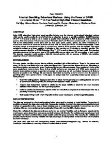
Number records in key value sets [FlattenWhole]
APPENDIX: FLOWCHART
Start
Transpose numeric fields into one record per value [FlattenPart]
Build list of SAS tables Select Table [ProcessFileList]
Transpose numeric fields into one record per key set [FlattenPart]
Sort by keys to WORK Library [ProcessFile]
Transpose character fields into one record per value [FlattenPart]
Determine Maximum Number of records per key value [ProcessFile]
Transpose character fields into one record per key set [FlattenPart]
Save table information to MEMBERS table [ProcessFile]
Yes
More than one record per key? [ProcessFile]
Merge numeric and character tables by keys [FlattenWhole]
File list exhausted? [ProcessFileList]
No
No
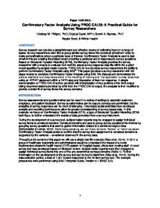
14
Yes
Next Page
From Previous Page
Merge relational files by keys
Open ODS spreadsheet
Print records of MEMBER table Print contents of flat table
Close ODS spreadsheet
Stop
15