Acta Agrophysica, 2005, 6(1), 261-272
ARTIFICIAL NEURAL NETWORKS IN COMPOSITIONAL ANALYSIS OF RAPESEED MEAL FROM NIRS – ASSESSMENT OF APPLICABILITY∗ Marek Wróbel1, Henryk Czarnik-Matusewicz2, Ryszard Siuda1 1
Institute of Mathematics and Physics, University of Technology and Agriculture ul. Kaliskiego 7, 85-796 Bydgoszcz e-mail:
[email protected] 2 Research Institute of Clinical Pharmacology, Faculty of Pharmacy, Medical Academy ul. Bujwida 44, 50-345 Wrocław
Ab s t r a c t . Near Infra-Red Spectroscopy (NIRS) is a rapid and cost-effective method widely used for the determination of chemical composition of agricultural products. Reflectance spectra recorded in near infra-red region for a set of samples of known composition are used for establishing calibration model by use of one of standard multivariate calibration methods, like MLR (multiple linear regression), PCR (principal component regression) or PLS (partial least squares). Multivariate calibration is a task that can be tried to be solved with artificial neural networks (ANNs) as well. The present paper is aimed at assessing the applicability of artificial neural networks as a tool for the determination of the content of main nutritional components of rapeseed meal: protein, dry mass, fibre and oil, on the basis of NIRS measurements. To the knowledge of the authors, no paper has been published on modelling of the dependence of chemical composition of rapeseed meal and NIR spectra with ANNs. Two most popular types of ANNs are tried in this work: multi-layer perceptron (MLP) and radial basis function (RBF). The obtained results show that chosen types of ANNs can provide models of performance comparable to that characterizing models built with MLR. K e y w o r d s : rapeseed meal, artificial neural networks, near infrared spectroscopy
INTRODUCTION
For many years one can observe wider and wider use of Near Infra-Red Spectroscopy (NIRS) in the determination of chemical composition of agricultural products, food, food components and beverages. The reasons behind this tendency are numerous and well known [11,20]. The main of them can be summarised under the headline cost-effectiveness. Over decades, two streams in the develop∗
The paper was presented and published in the frame of activity of the Centre of Excellence AGROPHYSICS – Contract No.: QLAM-2001-00428 sponsored by EU within the 5FP.
262
M. WRÓBEL et al.
ment and improvement of NIRS applications can be clearly seen: progress in instrumentation and progress in processing the results of measurements. Efforts within the latter stream, if directed towards extraction of chemical information, are well known as chemometrics. Chemometrics is closely related to many other branches of science oriented on the interpretation of real-world data, like applied statistics, artificial intelligence, and some others. As a consequence, chemometrics is a vital branch that still absorbs new ideas and methods. This can be also seen within the applications of NIRS in compositional analysis of food and food-related products. In particular, the potential of Artificial Neural Networks (ANNs) as a tool for extraction of chemical information from NIR spectra is an example of more recent efforts in chemometrics. The standard approach in chemical characterization of food with NIRS is to use one of the methods elaborated for purposes of multivariate calibration, such as MLR, PCR or PLS. However, it is always worth to evaluate the potential of any other possibility in order to confront the quality of the results it provides with the results coming from more standard tools. The aim of the present contribution is to evaluate the virtue of application of ANN as compared to the results that can be obtained by means of traditional methods for multivariate calibration [7] within a specific task defined as determining the chemical composition of rapeseed meal from NIRS. Two types of popular feedforward ANNs were chosen, i.e. with multi-layer perceptrons (MLP), and radial basis functions (RBF). PRINCIPLES OF ARTIFICIAL NEURAL NETWORKS
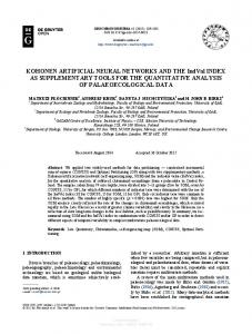
For many years ANNs have attracted much attention of workers from various branches. Consequently, huge literature on the subject exists. General and exhaustive introductions to the subject can be found in numerous handbooks, for instance in [12,13,15]; herein just the foundations of the most popular types of ANNs are presented and followed with a more detailed description of the present application. Figure 1 depicts the architecture of a simple ANN consisting of elements displayed in three functional layers. From the left, there are ni inputs (in the input layer) transmitting ni signals to each of nh neurons in the so-called hidden layer. The last layer consists of a single element, i.e. a single neuron in the output layer. In general, the number of hidden layers can be arbitrary as well as the number of neurons, no, in the output layer. The latter typically is equal to the number of dependent variables, while ni – to the number of input variables. The scheme of the architecture shown in Figure 1 is common for the types of ANNs that have been decided to be applied in the present work, i.e. to the types where the signals are transmitted in one direction without any feed-backs. This type of ANNs is called feed-forward nets. Within this category one can find some differences, first of all referred to the way in which neurons in hidden layer(s) transform signals from their inputs to their outputs. From this point of view, one
ARTIFICIAL NEURAL NETWORKS IN COMPOSITIONAL ANALYSIS
263
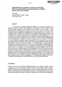
can distinguish two popular cases: multilayer perceptron (MLP), and radial basis functions (RBF), both chosen to be tried in the present work. Training of the ANN relies on adaptation of the values of some parameters (weights and biases in MLP, or centroids and widths in RBF). As the number of parameters to be adapted increases with the number of neurons, then rich architectures need more numerous training sets. Since the total number of the measured rapeseed meal samples is not very numerous in the present case study, it is reasonable to limit the number of neurons and to construct ANNs specific to each of rapeseed meal constituents. The net has to be trained in order to model in a satisfactory (in light of certain criteria) way the dependence between input and output variables. This unknown dependence is embedded in the data, and training (learning) results in finding a set of parameters of the net that enable the net to approximate the relationship between the inputs and outputs. Multilayer perceptron (MLP) Multilayer perceptron together with error back-propagation learning rule used in modelling of the dependency between input and output sets of variables create the most popular approach within applications of ANNs. Properties of this type of ANN are determined by the way in which particular neurons process their input signals into output signals. A single neuron participation in this processing can be schematically depicted as in Figure 2, and explained in several points: - each neuron accepts input signals xi and generates its output signal y, - each input has its weight, wi, which ascribes the importance to the information coming from the input, - each neuron has its bias (threshold value), w0, which influences the intrinsic activation of the neuron, ni
-
intrinsic activation of the neuron, s, equals to s = ∑ wi xi + w0 , i =1
- the output is y = f (s ) , where f(.) is the transfer function of the neuron. The transfer function can be of different shapes, either linear or non-linear. The most popular is the sigmoidal transfer function, either in its uni- or bi-polar variant, given by the formula 1 , λ>0 1 + exp ( − λs)
(1)
2 − 1, λ > 0 1 + exp ( − λs)
(2)
f(s) =
or f(s) =
respectively.
264
x1
M. WRÓBEL et al.
w11
fh
Fig. 1. The architecture of ANNs used in this work w1
fh
xi
w ji
fh
x1
w1
wj
w0
yˆ
∑
fo xi
wnh
+1
x ni
s
y f
wi wni
Fig. 2. Neuron model in MLP type nets x ni
wnh , ni
fh
The output signal of the whole net, yˆ , to an input vector x, of MLP-ANN with ni input neurons, one hidden layer with nh neurons, and one output neuron is (cf. Figs. 1 and 2) nh ni yˆ = f o w0 + ∑ w j f h ∑ w ji xi + w j 0 j =1 i =1
(3)
where f o and f h are transfer functions of output and hidden neurons, respectively. Training of a net with MLP starts with setting initial values of the weights and biases, usually at random. As a consequence, these parameters in the trained net may be not the same when the training is repeated.
ARTIFICIAL NEURAL NETWORKS IN COMPOSITIONAL ANALYSIS
265
Radial basis function (RBF) This category of ANNs uses transfer functions of radial shape, often Gaussian, adopted to each hidden neuron. Gaussian radial function for the i-th hidden neuron can be written as x − ci 2 (4) Φi ( x − c i ,σ i ) = exp − 2 2 σ i where x is the vector of input variables, ci and σi are the centroid and the width of the function, respectively. RBF-ANNs usually contain a single hidden layer, and the weights between the input and the hidden layers are set to unity. The output signal (cf. Fig. 1) is calculated as a weighted sum of the radial basis functions yˆ = ∑ wiΦi ( x − c i ,σ i ) nh
(5)
i =1
where nh is the number of hidden neurons, wi is the i-th weight between hidden and output layers. RBFs are known to allow modelling of non-linear dependencies with a linear approach, which ensures optimal weights for signals between hidden and output layers to be set for a given training set and architecture [9,19]. This means that after training the net reaches the same parameters for the same training data. By comparison of equations (3) and (5) one can see that radial functions act locally because their significant values occur close to ci only, while with increasing distance x − c i they fall rapidly. In MLP-ANN transfer functions act globally, because all the components of x influence the intrinsic activation of the neuron proportionally to the values of suitable weights. Hence, in nets with MLP processing of x with sigmoidal transfer function has a global character [12]. Modelling Typical tasks that appear when using ANN refer to: (i) pre-preparation of the data (see next section) and (ii) the size of the data set. Large enough data sets being available is the most desired situation, however very often the sets are not numerous enough to be simply split into training and prediction subsets that are needed to perform training (modelling) of the net and evaluation of the result. Details of the problems are extensively discussed in the literature (see, e.g. [4]). A large data set characterizes the modelled dependence more accurately and in more details. Moreover, such a set can be split into calibration and external test subsets at random, making the subsets likely independent. The latter property is not fulfilled when less numerous data set is split, since splitting needs special
266
M. WRÓBEL et al.
algorithms to ensure statistical similarity of both subsets. Because the number of samples was not large (NTOT = 69), duplex algorithm for splitting [16,17] was used and calibration subset of NC = 50 samples and external test subset of NTEST = 19 were formed. As the calibration set is not large enough, the so-called Monte Carlo cross-validation procedure [1] can be used in training of the net. This procedure selects a part of the calibration set as a training set and uses the remaining part as an internal test set and monitoring set. The latter set stops learning algorithm (socalled early stopping procedure [1,2] was used), then partial error RMSECV is calculated for the internal test set. This sequence is repeated 30 – 50 times, then total RMSECV is assumed as the mean of the errors obtained for all internal test sets. Finally, the net is tested on external test set in order to calculate RMSEP (see Tab. 1). In this work the training set included NTR = 40 samples, the monitoring and internal test set NMON = NCV = 5 samples, and the number of splits of training set equals NMC = 50. The Levenberg-Marquardt optimization method [2,5] was applied for setting weights in all learnings. Performance parameters used for the assessment of the models are listed and explained in the table below. Table 1. Parameters chosen for assessment of performance of models Name of performance index
Formula n
R2 coefficient of multiple determination
R2 =1−
∑ ( yˆ i =1 n
− yi )
2
i
∑ (y − y )
2
i
i =1
where n = NC for calibration set and n = NTEST for external validation subset.
∑∑ (yˆ N MC N X
RMSEC (CV) root mean squared error of calibration (cross-validation)
RMSEC, RMSECV =
i =1 j =1
− yij )
2
ij
N MC N X
where NX = NTR for RMSEC and NX = NCV for RMSECV N TEST
RMSEP root mean squared error of prediction
RMSEP =
∑ ( yˆ
− yi )
2
i
i =1
N TEST
RER y − y min ratio of the range to the standard RER = max error of prediction RMSEP ˆy i is the value of concentration of constituent for sample i predicted by the model from the spectrum, and yi is the value of concentration of constituent for sample i determined with the reference method.
ARTIFICIAL NEURAL NETWORKS IN COMPOSITIONAL ANALYSIS
267
For RBF-ANN, a frequently used approach is the regularization procedure [9] which results both in stabilization of the training process and avoiding of overtraining. In the present work, the so-called local ridge regression method was chosen for this purpose. Additionally, the forward selection procedure was used for establishing the optimal number (nh) of neurons in the hidden layer. The coordinates of objects from the calibration set were the possible centres (ci) and σi was common for all radial functions. Training of RBF-ANN does not need calibration set to be split into subsets, hence RMSECV was not calculated. DATA AND DATA PRE-TREATMENT
Data The set of data consisted of 69 reflectance near infrared spectra recorded for 69 rapeseed meal samples of chemical composition determined with approved chemical methods [8] (for more details see accompanying paper [7]). Determining chemical composition of the samples from NIR measurements, i.e. contents of four compounds (protein, dry mass, fibre and oil), was the goal of modelling with ANNs. Data pre-treatment Multiple scatter correction (MSC): The MSC is the most commonly used pretreatment of NIR reflectance spectra aimed at reducing multiple scattering effect present when measurements come from granular samples [6]. MSC is performed on subsets of original spectra selected for calibration and for external test sets. The spectra of external test sets are MSC transformed by use of the mean spectrum obtained from the MSC of the calibration set. Selection of input variables: The number of wavelengths in the spectra is equal to 700, and it is too large for direct use of all of them as input variables for ANN. Therefore, a reduction of the number of input variables to a subset of reasonable size, e.g. to some tens, is needed. With this aim, the so-called CVU method, recently proposed for wavelength selection in multivariate calibration [14], has been applied. Scaling of input variables: This step is necessary in order to avoid the situation when a large change in neuron intrinsic activation, s, can result in a low change of its output because of saturation in transfer function (details on scaling can be found in [4]). In this paper the input variables xi were scaled (after centring) to the range of (-1,1), i.e. to the quasi-linear range of non-linear transfer function. Scaling of the data from the external test set used the scaling parameters determined on the calibration set. Since transfer function processes signal s de-
268
M. WRÓBEL et al.
pendent also on weights, it is recommended to chose initial weights with a special method, e.g., the Nguyen-Widrow method [5,18]. Also output signals (reference data) have to be scaled. When the transfer function of output neurons is nonlinear, the range recommended for scaling is 0.2 to 0.8, while linear functions usually make scaling not necessary, although in some cases scaling is recommended as well [4]. In this paper the reference data (contents of constituents) were not range scaled. For RBF-ANN results of scaling and centring of the input data can be effectively replaced with a suitable choice of centroids and widths in the transfer functions. COMPUTATIONS AND RESULTS
Computer simulations of NN were performed with Neural Network toolbox Matlab 6.5 package [2]. Splitting of the data was performed with the Calibration toolbox [17]. Building calibration models by means of RBF was carried out with Matlab Routines for Linear Neural Network toolbox [10]. Remaining calculations were made with software developed by the authors. The first task for MLP-ANNs was to determine the optimum architecture. For a given number of hidden neurons, changed steeply between 2 and 10, the numbers of neurons in the input layer (between 2 and 10) were tested. For each architecture, calibration was performed fivefold, then the mean and standard deviation of the performance parameters of the obtained models were calculated. The transfer functions used in the hidden layer were uni-polar sigmoid (eqn. 1) and the transfer functions in the output layer were linear. In the RBF-ANNs the value of σi was determined by optimisation of the models obtained for ni ∈ {2, 3, ..., 10} while σi changed between 0.02 to 2 with step of 0.02. The calibration and external test sets were the same as those used for MLP. Mean values and standard deviations of performance parameters of the models obtained for five series of trainings (mean values for protein were calculated for four trainings only since in one training the result was far from the remaining ones) are listed in Table 2. Parameters obtained for fibre were less reproducible both for MLP and RBF (see Tab. 3). The most important parameter is RER (see Tab. 1) as it shows the relation between errors of the model and the range for content of the constituent. Comparison of this parameter for both types of networks does not show noticeable differences, except for oil, where RBF gives a considerably better (larger) value. Optimal size of MPL nets were low, especially in the hidden layer where 2 or 3 neurons only were necessary. The number of inputs was the greatest for the modelling of protein and oil, however 10 and 7 inputs, respectively, are not very high. It is worth pointing out that for dry mass and fibre only 2 inputs were needed
ARTIFICIAL NEURAL NETWORKS IN COMPOSITIONAL ANALYSIS
269
(i.e. only 2 wavelengths) in order to obtain quite satisfactory models. Comparison of the architectures for MPL and RBF nets shows considerably greater number of neurons in the hidden layer. This can be expected because of general properties of this type of ANN [3]. One can also see that the number of inputs in RBF weakly depends on modelled constituent and ranges between 6 and 8. Table 2. Mean values and standard deviations of performance parameters for models from MLP-ANN Constituent
Model
Set
ni-nh-no
protein
10-2-1
dry mass
2-2-1
fibre
2-3-1
oil
7-3-1
cal. test cal. test cal. test cal. test
R2 mean 0.89 0.86 0.95 0.96 0.84 0.78 0.98 0.96
std. 0.01 0.02 0.00 0.00 0.00 0.02 0.00 0.00
RMSEC (%) mean std.
RMSECV (%) mean std.
RMSEP (%) mean std.
mean std.
0.94
0.03
1.00
0.04
0.95
0.05
10.8
0.6
0.26
0.01
0.29
0.01
0.32
0.01
23.7
0.5
0.84
0.06
1.01
0.16
0.88
0.05
10.1
0.5
0.16
0.01
0.18
0.01
0.35
0.02
24.4
1.6
RER
Table 3. Performance parameters for models from RBF-ANN R2
Model ni-nh-no
cal.
test
protein
8-7-1
0.86
dry mass
7-3-1
fibre oil
Constituent
RMSEC (%)
RMSEP (%)
RER
0.85
0.94
0.97
10.5
0.93
0.95
0.29
0.36
20.8
7-15-1
0.97
0.86
0.34
0.71
12.5
6-10-1
0.98
0.98
0.16
0.23
36.6
Parameters of the models obtained with both types of ANNs are similar to the results obtained with MLR (Tab. 4). One can see from the above table that fibre and oil need considerably greater numbers of wavelengths to be involved in MLR models than when neural networks are used for modelling. The best modelling consti- Table 4. Results of MLR method (from ref. [8]) No. of tuent with all methods of modelling Constituent R2 RER wavelengths considered in the present work is oil. Very satisfactory models could be obprotein 0.82 9.4 9 tained also for dry mass, while remaindry mass 0.92 21.2 4 ning constituents provided noticeably fibre 0.88 13.0 15 less valuable models, although still oil 0.98 42.2 11 acceptable for purposes of quality control.
270
M. WRÓBEL et al.
CONCLUSIONS
Comparison of the models provided by two types of networks shows that MLP-ANNs need simpler architecture. An exceptionally low number of input variables is necessary when dry mass and fibre are modelled. RBF-ANNs are more extended, especially in the hidden layer. On the other hand, for the case of oil, this type of net provided a model of very good performance. Therefore, the obtained results do not indicate any clear advantage of any one type of ANN. Comparison of the results of ANNs and MLR shows the models are similar, with the exception of oil, where RER from MLR is considerably better. However, the number of wavelengths needed in MLR tends to exceed the number of inputs in MLP-ANNs, like in the case of RBF-ANNs. To conclude, although the presented results for modelling of the content of four compounds in rapeseed meal from NIRS are preliminary, they show that calibration models that can be obtained from linear multivariate calibration are of better performance compared to the results from ANNs. There can be several reasons for this situation: - not large enough sets of data, - not optimal choice of the methods for both input variables selection and scaling of the output signal, - common widths in transfer functions for RBF-ANNs. Suitable modifications made according to the points listed above can be expected to result in improvement of the ANN’s models. REFERENCES 1.
2. 3.
4. 5.
6. 7. 8.
Adamczak R.: Application of neural networks for classification experimental data (in Polish). doctor’s thesis, Department of Computer Methods, Nicholas Copernicus University, Toruń, Poland, 2001, http://www.phys.uni.torun.pl/publications/kmk/01phd-ra.pdf Demuth H., Beale M.: NN Toolbox User's Guide. The MathWorks, Inc., 2003. Derks E.P.P.A., Sánchez Pastor M.S., Buydens L.M.C.: Robustness analysis of radial base function and multi-layered feed-forward neural network models. Chemom. Intell. Lab. Syst., 28, 49-60, 1995. Despange F., Massart D.L.: Neural networks in multivariate calibration. Analyst, 123, 157R178R, 1998. Eagen W.J., Angel S.M., Morgan S.L.: Rapid optimisation and minimal complexity in computational neural network multivariate calibration of chlorinated hydrocarbons using Raman spectroscopy. J. Chemom., 15, 29-48, 2001. Geladi P., McDougall D., Martens H.: Linearization and scatter-correction for near-infrared reflectance spectra of meat. App. Spectrosc., 39, 491-500, 1985. Jankowski J., Czarnik-Matusewicz H., Siuda R.: Comparison of MLR and PLS models in compositional analysis of rapeseed meal from NIR, Acta Agrophysica, 91-102, 2205. Official Methods of Analysis, 16th edition on CD-ROM, AOAC, Arlington, Virginia, USA, 1995.
ARTIFICIAL NEURAL NETWORKS IN COMPOSITIONAL ANALYSIS 9. 10. 11. 12. 13. 14. 15.
16. 17. 18. 19. 20.
271
Orr M.J.L.: Introduction to radial basis function networks. Technical Report, Centre for Cognitive Science, Edinburgh University, 1996, http://www.anc.ed.ac.uk/~mjo/intro/intro.html Orr M.J.L.: Matlab routines for subset selection and ridge regression in linear neural networks. ver. 1.013, 1997, http://www.anc.ed.ac.uk/~mjo/software/rbf.zip Osborne B.G., Fearn T.: Near-infrared spectroscopy in food analysis. Longman Scientific and Technical, New York, USA, 1986. Osowski S.: Neural networks for information processing (in Polish). Printing House of the Warsaw University of Technology, Warszawa, 2000. Otto M.: Chemometrics. WILEY-VCH, 1999. Siuda R.: A simple approach to input variable selection in multivariate calibration. Submitted to J. Chemometrics. Smits J.R.M., Melssen W.J., Buydens L.M.C., Kateman G.: Using artificial neural networks for solving chemical problems. Part I. Multi-layer feed-forward networks, Chemom. Intell. Lab. Syst., 22, 165-189, 1994. Snee R.D.: Validation of regression models: methods and examples. Technometrics, 19(4), 415-428, 1977. The CALBRATION toolbox, FABI, Vrije Universiteit Brussel, http://www.vub.ac.be/fabi/ Walczak B.: Neural networks with robust backpropagation learning algorithm. Anal. Chim. Acta, 322, 21-29, 1996. Walczak B., Massart D.L.: Local modelling with radial basis function networks. Chemom. Intell. Lab. Syst., 50, 179-198, 2000. Williams P.C., Norris K.H. (Eds.): Near-infrared technology in the agricultural and foods industries. American Association of Cereal Chemists, Inc., St. Paul, Minneapolis, USA, 1987.
SZTUCZNE SIECI NEURONOWE W ANALIZIE SKŁADNIKOWEJ ŚRUTY RZEPAKOWEJ NA PODSTAWIE NIRS – MOśLIWOŚCI ZASTOSOWAŃ Marek Wróbel1, Henryk Czarnik-Matusewicz2, Ryszard Siuda1 1
Instytut Matematyki i Fizyki, Akademia Techniczno-Rolnicza ul. Kaliskiego 7, 85-796 Bydgoszcz e-mail:
[email protected] 2 Zakład Farmakologii Klinicznej, Wydział Farmacji, Akademia Medyczna ul. Bujwida 44, 50-345 Wrocław S t r e s z c z e n i e . Spektroskopia w bliskiej podczerwieni (NIRS) jest szybką i wydajną metodą, szeroko wykorzystywaną do określania składu chemicznego produktów rolniczych. Widma odbiciowe zarejestrowane w obszarze bliskiej podczerwieni dla zbioru próbek o znanym składzie wykorzystuje się do ustalenia modelu kalibracyjnego przy uŜyciu standardowych metod wielowymiarowej kalibracji, takich jak MLR, PCR lub PLS. Wielowymiarowa kalibracja jest zadaniem, które moŜe być równieŜ rozwiązane przez sztuczne sieci neuronowe (ANNs). Celem tej pracy jest ocena moŜliwości zastosowań sztucznych sieci neuronowych jako narzędzia do określania zawartości głównych składników odŜywczych śruty rzepakowej: białka, suchej masy, włókna i tłuszczu na podstawie pomiarów NIRS. Według wiedzy autorów w literaturze nie są znane prace na temat modelowania zaleŜności składu chemicznego śruty rzepakowej na podstawie widm NIR przez ANNs. W pracy zastosowano dwa najpopularniejsze typy sztucznych sieci neuronowych:
272
M. WRÓBEL et al.
perceptron wielowarstwowy (MLP) i sieć z radialnymi funkcjami bazowymi (RBF). Otrzymano rezultaty w postaci modeli, których jakość jest porównywalna z jakością modeli moŜliwych do uzyskania za pomocą MLR. S ł o wa k l u c z o w e : śruta rzepakowa, sztuczne sieci neuronowe, spektroskopia w bliskiej podczerwieni