2D Image Reconstruction and Zooming with Simultaneous Edge

2D Image Reconstruction and Zooming with Simultaneous Edge Preservation and Blur Christopher Hazard Biomedical Engineering, Ohio State University and Jian Huang, Roger Crawfis Computer and Information Science, Ohio State University Columbus, OH 43210, U.S.A.

ABSTRACT This paper presents a method of reconstructing twodimensional images at varying spatial resolutions while preserving edge information and allowing for blurring. It is often the case that a user would like to zoom in on certain areas of an image. Such a zoom operation requires a reconstruction of the data to provide values at the resampled pixel locations. Standard reconstruction methods use a spatially invariant reconstruction kernel such as a Gaussian or spline to perform this resampling. These reconstructions result in blurred edges and preserve noise artifacts. The reconstruction method described in this paper uses a spatially varying kernel to allow preservation of edges at the various resolutions. In addition the reconstruction allows the user to specify regions to blur in the reconstructed image. This allows the user to display magnified images in which the edge locations are preserved and unimportant areas are deemphasized. This reconstruction scheme has been applied to several test data sets. The resulting images demonstrate the algorithm’s ability to magnify an image while preserving edges and blurring unwanted detail. Keywords: Image Reconstruction, Zoom, Edge Preservation, Blur.

1. INTRODUCTION A common task in image processing is reconstructing an image at a higher resolution than the acquired data. Such a zoom operation requires a resampling of the data to provide values at each pixel location. If the underlying continuous function is band limited and the resulting input image is sampled at a sufficient rate it is theoretically possible to reconstruct the continuous function exactly. However, such a reconstruction requires an infinite filter which is not realizable and a good approximation is computationally expensive. Furthermore, for many applications the desired function is not band limited, or has frequencies higher than those in the lowpass image. As a result, simpler filters are employed in reconstruction. Standard reconstruction methods use a spatially invariant kernel such as a Gaussian or spline to reconstruct the underlying continuous function and resample at the new locations. Additionally, the range of influence of the reconstruction kernel is limited to allow a practical implementation of the filter. Max determined a reconstruction

kernel that was optimal for reconstructing a uniform image with a spatially invariant kernel [1]. This kernel is limited in extent and can be easily computed. There are many ways in which an image conveys information, but edges are perhaps the most important. The edge between healthy tissue and cancerous cells is just one example of the importance of edges. These edges may be ill-defined in the low-passed image, and the radiologist or various edge detection schemes may be needed to determine their locations. Our goal is to preserve and enhance edges in a magnified image. Since the optimal kernels of Max and others are designed to reconstruct a uniform image they tend to blur edges by averaging out the discontinuity. Here, we associate with each data point a spatially varying reconstruction kernel, to allow reconstruction of functions with sharp edges. Another problem in image display is noise. When a user identifies noise in an image it is often intentionally blurred. Unfortunately the intentional blur that de-emphasizes noise will also destroy the edges. There is a need for a display algorithm that allows for blur, but at the same time retains the important edge information. Since we specify a unique reconstruction kernel for each pixel, we can include specific information to simultaneously preserve the edges while blurring. Much of the image processing literature concerning edge enhancement with noise removal is focussed on iterative algorithms that converge to a solution slowly [2,3,4]. These algorithms require multiple passes through the data and are not well suited for use in a simple zooming algorithm for image display. These algorithms are also concerned with edge enhancement without prior edge identification. Often times the location of the edges can be determined by the user and then display is the only issue. In this paper we are concerned with a simple and fast display algorithm and we assume that the edge locations are either known, user defined or precalculated by an edge detection routine. Similarly, we assume that the suspected noise pixels have been identified. This paper focuses strictly on the reconstruction and resampling of the image using this information. Huang, Crawfis, and Stredney have recently done work to preserve and enhance edges in the context of volume rendering using splats [5]. The work presented in this paper is the practical application of the techniques developed for the

volume rendering edge preservation, to the simpler case of 2D image reconstruction.

associated with a pixel that is within a single pixel length of the edge. A secondary kernel is associated with a pixel

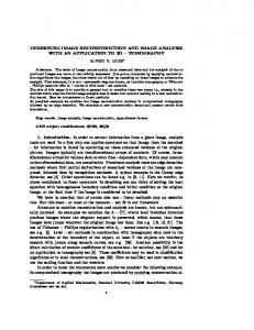
2. ALGORITHM Edge Location Orientation

Input Image Zoom Algorithm

Kernel Type Blur Level

Zoom Level

Zoom Image

Figure 1: Black box depiction of Zoom algorithm with inputs and output. Figure 1 is a black box representation of the zoom algorithm. The algorithm requires several inputs in order to produce the output zoomed image. The input image is the image for which enlargement is desired. In addition to this image four (or more) two dimensional arrays are also necessary. The necessary arrays are edge location, edge orientation, kernel type, blur level, and possibly edge strength. These arrays correspond to parameters used in the zoom algorithm and each is described below. Additionally the level of zoom must be specified. The zoom level is the magnification factor and was fixed at a level of three for the images in this paper.

Figure 2: Max’s Optimal 2D Kernel located more than one pixel length but less than two pixel lengths from the edge. These secondary kernels are necessary to ensure proper reconstruction in the regions where the reconstruction kernels overlap. Pixels greater than two units away are assumed to have negligible contributions to edge and have unaltered kernels associated with them. Since and edge represents the transition from a region of relatively high intensity to a region of relatively low intensity, we use high or low to designate which side of the edge the pixel associated with the kernel is located. Figure 3 summarizes these designations. High

It is assumed that the input parameter arrays are available to the zoom algorithm. Edge location and orientation can be determined using standard image processing algorithms for edge detection or the user can manually trace the edges. Kernel type and blur level assignments can also be done manually or auxiliary algorithms can be used to automatically make such assignments. For sharp transitions in 2D contour filling algorithms, the edge information can be approximated using the gradient of the input field. The edge location and orientation information is then used to vary the kernel used for reconstruction of the higher resolution image. The kernels near an edge are modified to artificially enhance the edge by re-mapping a standard kernel using a non-linear transformation. The non-linear mapping function used is that presented by Huang, Crawfis and Stredney [5]. A detailed analysis of this non-linear stretching function is given in the reference and is beyond the scope of this paper. Huang used the optimal reconstruction kernel for splatting, as presented by Crawfis et. al. [6], as the base kernel. This kernel is optimized to reconstruct a uniform 3D volume. Since this paper is concerned with 2D images, the Crawfis kernel is not appropriate. Figure 2 shows a similar optimal 2D kernel as presented by Max [1], which we have used as the base kernel for the reconstructions. This basic kernel is modified by a stretching function to create new kernels for edge enhancement. There are four modified edge kernels in the implementation used for the reconstructions in this paper. In the language of Hunag, Crawfis and Stredney [1], the kernels are labeled as primary or secondary and high or low. A primary kernel is

Low Primary Kernel

Edge

Secondary Kernel

Figure 3: Kernel designations The modified kernels are controlled by three parameters: edge location, edge strength, and edge orientation. Edge location refers to the position of the edge relative to the original image samples. Edge location is specified as a positive or negative distance to indicate whether the pixel is on the “high” or “low” side of the edge. Edge strength determines how much of an influence the edge has on the reconstruction. That is, it determines how sharp or crisp the resulting edge will be. This allows for a variety of edge profiles. Edge orientation refers to the direction of the edge in the plane of the image. Arrays of each of these parameters are used as input to the zooming algorithm. A blur function was also added to allow the user to blur noise while preserving the edge. A blur is achieved by redistributing the energy in the kernel over a larger region of the final image. For this paper, the blur was done by stretching the optimal kernel prior to applying the edge stretching function. The base kernel is radially symmetric, thus the stretching is just a rescaling of the radial axis. If g(r) is our kernel function, we use g(r’) where r’ is a constant times r. The constant is chosen for each level of blur. Since the constant is chosen to be less than one, the energy of the

kernel is spread out over a larger number of pixels in the image. Image reconstruction involves stepping over each of the original image samples, selecting the appropriate kernel and then adding that kernel to the new image buffer. One advantage of the spatially invariant kernels used in standard reconstruction is that the kernel can be calculated once and then used for every sample in the image. This allows for very fast reconstruction. In order to obtain similar reconstruction times using the spatially varying kernels, they must also be pre-calculated. This requires that kernels be calculated for discrete values of the controlling parameters. If done for a sufficiently large number of samples in the parameters, the discretization does not significantly affect the quality of the reconstruction. The pre-calculated kernels are then stored in a lookup table indexed by edge location, edge strength, and blur. A section of the lookup table is shown in the Figure 4.

Figure 5: Simple example image (8 x 8 pixels)

Non-edge

Secondary-high

Primary-high

Primary-low

Secondary-low Figure 4: Portion of kernel lookup table

Figure 4 shows the five kernels (non-edge, secondary low, primary low, primary high, and secondary high) for several levels of blur. Blur increases from right to left. Only a single edge strength and edge location is depicted in the figure. The table for this paper was built to provide a three times magnification.

Figure 6: Reconstruction with single optimal kernel

Additionally, rotations of the kernels can be pre-calculated or done using texture mapping hardware. Reconstruction is performed by selecting the correct kernel from the table based on the calculated and user specified parameters for each sample in the original image. This kernel is then weighted by the sample value, shifted to the appropriate location, resampled to the desired resolution, and added to the output image. The final image is obtained by repeating this process for each of the original image samples. 3. SIMPLE EXAMPLE Figures 5 through 11 show a simple example of a reconstruction that illustrates the ability of the algorithm to preserve edges while allowing for simultaneous blur. Figure 5 shows an example data set exhibiting a strong edge. The image consists of a dark and light band. The dark region has a

Figure 7: Reconstruction with enhanced edge kernels

Figure 8: Reconstruction of spike image with single optimal kernel

Figure 9: Reconstruction of spike image with enhanced edge kernels pixel intensity of 10 and the light region has a pixel intensity of 100. This continuous function is sampled to only 8 x 8 pixels, or discrete data points, and used as input for the subsequent tests. Magnifying the image three times and reconstructing results in a 24 x 24 pixel version of the image. Figure 6 shows the reconstruction if the spatially invariant optimal kernel is used. Note that distortion around the periphery is expected because the reconstruction used zeros for values of samples outside the original image. Figure 6 reveals that the edge is smeared by the simple single kernel reconstruction. Figure 7 shows the reconstruction with the modified edge kernels. It was assumed that the edge was located half way

Figure 10: Single kernel reconstruction of spike image with blur

Figure 11: Edge kernel reconstruction of spike image with blur between the pixels in the original image for the reconstruction. The effect of edge strength was not explored in this example. Mach banding is present in the image as a result of discontinuities in the higher order derivatives. The edge kernels were designed to be only C1. The figure reveals that the edge is crisper with the edge enhanced kernels. To simulate noise in the image we place a spike with a value of 80 in the dark region of our sample image at pixel location (4,4). Figures 8 and 9 are the reconstructions using the single spatially invariant kernel and edge kernels respectively, for the sample data set with a single spike. The single kernel reconstruction blurs the noise and edge. This blurring results from the averaging nature of the

magnification processes. When the edge kernels are used the edge is maintained while the spike is blurred by the averaging process. In addition to the natural blur caused by the magnification process, the user may wish to blur certain regions of the image. This additional blur is achieved by spreading the energy of the kernel over a larger region and was described previously. Figures 10 and 11 show the spike image with additional blur specified at the spike pixel location. Figure 10 uses the single kernel reconstruction and Figure 11 uses the edge kernels. These images reveal the ability of the reconstruction technique to maintain the edge and to blur the noise. 4. CIRCLE EXAMPLE The example in the previous section had only horizontal edges and thus no rotation of the kernels was necessary. In this section a more complicated but still constrained example is presented. In this section the image is a circle with a 25 pixel radius centered in a 100 x 100 pixel image. The pixel intensities inside the circle are 100 and the pixel intensites outside the circle are 10.

Figure 13: Reconstruction of circle with single kernel

Figure 12: Edge kernels assignments. Rings from inside to out (dark to light) are: secondary high, primary high, primary low, and secondary low. The circle data set reveals some of the challenges of implementing the edge kernel algorithm in data sets with varying edge directions. All images are cropped for display.

Figure 14: Reconstruction of circle using edge kernels

Figure 12 shows how the edge kernels were chosen for the reconstructions that follow. The rings from the inside to out are: secondary high, primary high, primary low, and secondary low. There is some ambiguity in the assignment of these kernels. Since the edge is not a straight line, artifacts are introduced into the reconstructions.

After magnification the resulting images are 300 x 300 pixels. A reconstruction using the single optimal kernel is shown in Figure 13. The edge of the circle is fuzzy in this image. Figure 14 shows the reconstruction using the edge kernels. The edge is crisp, but artifacts from the kernel selection ambiguity are seen as bright and dark regions along the edge. Correcting these is the subject of future investigations.

In addition to the kernel types, the edge location and edge direction must be specified for each pixel in the original image. These specifications can be determined for this artificial experiment, but can be difficult for experimental data or acquired images. Where manual traces exist, or an image is contoured, accurate edge information is available.

Next we added Gaussian noise with zero mean and a standard deviation of approximately 35 to our original image. Additionally two levels of noise were explored simultaneously in the single image. The left half of the image has a 30% probability of noise and the right half has a 70% probability of

Figure 15: Noise infected image of circle

Figure 16: Reconstruction using blur and single kernel

noise. This means that in left half of the image each pixel has a 30% chance of having noise added to that pixel value. Similarly the each pixel in the right half of the image has a 70% chance of having noise added to the image. Figure 15 shows this noise infected image. The magnified reconstructions of this image using the single kernel and the edge kernel show results similar to the simple example in the previous section. The edge is better represented by the edge kernels and the noise is somewhat blurred by the averaging process. To lessen the effect of the noise an additional blur is again used. If the blur level is chosen to be very large the effect of the edge kernels is diminished, but for moderate blur levels the edge kernels allow for noise blurring with edge preservation. Figure 16 shows the noisy image magnified using the single optimal kernel with some additional blur. Figure 17 shows the same image made using the edge kernels. The blurring has de-emphasized the noise in both images. The edge is crisp in the image made using the edge kernels. This further demonstrates the reconstruction algorithm’s ability to allow simultaneous blur and edge preservation. 5. PROBLEMS AND FUTURE WORK The examples in this paper have demonstrated the ability of the edge kernels to provide sharp edges in zoom images. Additionally the examples showed simultaneous blur and edge preservation in these zoomed images. It should be noted that this procedure can be used to allow magnification to any level. The algorithm uses edge location and orientation information that may not be easily obtained. For the contrived examples in this paper the edge location and orientation could be easily calculated. In a real image this is not the case. The user may specify the edge location, but orientation must still be

Figure 17: Reconstruction with blur using edge kernels calculated. A robust orientation calculation needs to be investigated. The effect of using different edge strengths was not explored in the examples in this paper. The edge strength parameter is part of the stretching functions developed by Huang et. al. [5]. A single value was used for all the reconstructions in this paper. Varying this parameter may allow for more control over the edge and may allow higher levels of blur with simultaneous edge preservation. Finally, the reconstruction process assumes linear edges, or C1 curves with low curvature. Corners are not addressed here. The artifacts in the circle images are due to the fact that

curvature is not included in the kernel designs. Including such curvature information in the kernels is an area for future research. 6.

ACKNOWLEDGEMETNS

The authors would like to thank Naeem Shareef for many insightful comments and corrections to the manuscript. 7. REFERENCES [1] N. Max, "An Optimal Filter For Image Reconstruction," Graphics Gems II, Academic Press, 1991:101-104. [2] M. Nitzberg, T. Shiota, "Nonlinear Image Filtering with Edge and Corner Enhancement," IEEE Transactions on Pattern Analysis and Machine Intelligence, August 1992;14(8):826-832. [3] A Lev, "Iterative Enhancement of Noisy Images," IEEE Transactions on Systems, Man and Cybernetics, June 1977;SMC-7(6):435-442. [4] S. Ranganath, "Image Filtering Using Multiresolution Representations," IEEE Transactions on Pattern Analysis and Machine Intelligence, May 1991;13(5):426-440. [5] J. Huang, R. Crawfis, D. Stredney. "Edge Presrvation in Volume Rendering Using Splatting," To appear in Proceedings 98 Symposium on Volume Visualization, ACM SIGGRAPH Press. [6] R. Crawfis, N. Max, "Texture Splats For 3D Scalar And Vector Field Visualization," IEEE Visualization ’93 Proceedings, October 1993:261-267 .