X-ray Computerised Tomography (CT) attempts at reconstructing a 3D struc- ... follow a simultaneous reconstruction and segmentation (SRS) approach to pro-.
Simultaneous Reconstruction and Segmentation of CT Scans with Shadowed Data F. Lauze1 and Y. Qu´eau2 and E. Plenge1 1
Department of Computer Science, Universtity of Copenhagen 2 Computer Vision Group, TU M¨ unchen
Abstract. We propose a variational approach for simultaneous reconstruction and multiclass segmentation of X-ray CT images, with limited field of view and missing data. We propose a simple energy minimisation approach, loosely based on a Bayesian rationale. The resulting non convex problem is solved by alternating reconstruction steps using an iterated relaxed proximal gradient, and a proximal approach for the segmentation. Preliminary results on synthetic data demonstrate the potential of the approach for synchrotron imaging applications.
1
Introduction
X-ray Computerised Tomography (CT) attempts at reconstructing a 3D structure from a set of planar projections that consist of attenuated measurements of X-rays across an object. In many domains, especially material sciences and geosciences, this reconstructed structure is often a building block for segmentation, which is further used to analyse some physical properties of the sample, such as porosity and tortuosity, or to perform some numerical simulations. Traditionally, and because of its low cost, Filtered Back Projection reconstruction (FBP) is performed, followed by segmentation. This has the disadvantage to propagate reconstruction errors in the segmentation. Other approaches have thus been proposed that do not decouple these steps. Discrete tomography [1] reconstructs an image with a small finite number of values, while Yoon et al. reconstruct a segmented image, using a level set approach [12]. In this work we follow a simultaneous reconstruction and segmentation (SRS) approach to produce both reconstructed image and its segmentation. This approach was first proposed by van Sompel and Brady [10], using a Hidden Markov Measure Field Model (HMMFM). Another was proposed by Ramlau and Ring in [8]. Romanov et al. [9] assumed that information about the segmentation is known in the form of prior knowledge on the parameters of a Gaussian Mixture Model for intensity distribution, and some partial convexification is performed. A Potts-Model based algorithm was proposed by Storah et al. in [11]. The present work is somewhat similar, though we place ourselve in a limited Field of View situation, where the detector extent is less than the object diameter. Algebraic Reconstruction Techniques (ART) are know to perform properly ([7], Chap VI), though an extra difficulty is that the signal may be partially blocked at certain angles, a situation
Fig. 1. Acquisition setup. Left: device holding the sample to be imaged. Right: limited Field of View and obstacle.
somewhat similar, but not identical to limited-angle tomography. FBP solvers can also reasonably deal with limited field of view by proper extension of the sinogram data (see also [7], Chap. VI), however, noise is still propagated and the presence of holes in the sinogram produces potentially severe streak artifacts in the reconstruction affecting thereafter the segmentation quality. One of the reasons for these streak artifacts is the fact that the absence of measurements is interpreted as a zero-measurement in FBP. Ongoing work on extending microlocal analysis [5] from the limited angle problem to this type of sinogram missing data is also providing clues on potential singularities arising from them.
This work is targeted towards Synchrotron X-Ray tomography, as often the case in material science. This means a simple, parallel beam geometry. We come back to the SRS problem where we attempt to estimate all parameters during the reconstruction and segmentation process. A clear modelling of what is available allows to properly take into account missing data, both for FoV and unrecorded data. Spatial regularisation, via Total Variation minimisation, and positivity constraints reduce noise and artifacts, providing an inpainting-like mechanism for the missing data. We couple it to a segmentation term which, in the reconstruction phase, also acts as a reaction towards specific values. Because out of the FoV, reconstructed values are not reliable, the segmentation is run only inside the FoV.
The paper is organised as follows. Section 2 formalises SRS with limited field of view and occluding geometry as a Bayesian inference problem. This yields an energy-minimisation formulation which is numerically tackled in Section 3. Starting from a rough initial reconstruction and segmentation obtained by standard methods, the proposed algorithm iteratively refines the reconstruction, given the current segmentation, and then the segmentation, given the current reconstruction. Both these steps are efficiently achieved by lagged proximal iterations. The preliminary results presented in Section 4 confirm that this joint approach is promising, in comparison with the standard sequential strategy.
2
Statement of the problem
For a monochromatic X-ray travelling along a line L, Lambert-Beer’s law asserts that � Z � Z I0 IL = I0 exp − f (x) dx ⇐⇒ yL := log = f (x) dx (2.1) IL L L where I0 is the initial intensity and f the attenuation coefficient function. Recovering f accounts thus to solving (2.1) for f when we have observed (yL )L . More precisely, the Radon transform R : L1 (D) → L1 (S1 × R) of a function f is defined as Z Rf (θ, s) = f (sθ + y) dy, θ ∈ S1 , s ∈ R. (2.2) θ⊥
with D a bounded domain of R2 , S1 the unit circle of R, and θ⊥ the line orthogonal to θ. The well celebrated inversion formula proven by Radon in 1917 states that when f is smooth with compact support, it can be recovered from its Radon transform by the inverse Radon transform: Z Z ∞ ∂ 1 ∂s Rf (θ, t) dtdθ. (2.3) f (x) = 2 4π S1 −∞ x · θ − t This inversion is however ill-posed, and in our setting, we observe only Rf (θ, s) for values (θ, s) in a potentially complex sub-domain of S1 × R, as illustrated in Fig. 2. Filtered backprojection (FBP) is used to stabilise the inverse Radon transform, and relatively simple tricks can deal with the limited Field of View problem in the (FBP) settings. The shadowing caused by the presence of metallic bars induces however serious artifacts in FBP. This has motivated us to follow a discrete, direct approach. Notations. We start by introducing notations used in the sequel. In the 2dimensional setting, the sought function f can be viewed as a discrete N ×N → R image x on a regular square grid, called tomogram and represented as a vector 2 of RN . It is assumed to be large enough to cover the object we want to image. Each xn , n = 1 . . . N 2 , satisfies xmin ≤ xn ≤ xmax
(2.4)
with xmin ≥ 0, xmax ≤ +∞. This is a simple box constraint and we denote by C 2 the box [xmin , xmax ]N . In the 3D setting, x would be a N × B × P discrete image, with similar box constraints. Yet, in this preliminary work we restrict ourselves to the 2D case. Because we are in the parallel beam geometry setting, each angular projection is inherently 2D to 1D. Assume ` directions and a detector array of length d with M elements, where d is larger that the diameter of the object under scrutiny. Our aim is to recover the image x from samples of the Radon transform of the underlying attenuation function f , which form an ` × M discrete image called sinogram, and represented as a vector y ∈ R`M . The corresponding projection
2
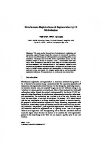
matrix / discrete Radon Transform R is thus an element of R`M ×N such that the sinogram is obtained as y = Rx. (2.5) This is a discrete analogue to the standard FBP setting. We choose here a simple model where entry Rij represents the contribution of grid element j to the line-ray encoded by i, as for instance the length of the intersection of this line and the grid element. Other less local representations can be chosen, see [4] for instance, for discussions on the generation of the discrete Radon transform matrices. When the detector array has a length d0 smaller than the object diameter, some parts of the object are not traversed by X-rays, or these rays are not recorded. If assuming the same resolution as for building R, the resulting projection matrix Q is made of a subset of lines of R. With m rays recorded per view, 2 Q is a R`m×N matrix obtained from R by a linear projector PF ∈ R`m×`M . The reduced sinogram y F is y F = PF y. In the situation described in Figure 1, the geometry of the missing data in the sinogram will vary according to the ratio between bar radius and detector extent. This is easily computed by projecting orthogonally the disks along the detector, at each angle. Figure 2 illustrates this in two extreme cases, a very large and a very narrow detector.
Fig. 2. Sinogram geometry induced by the occluding geometry of the bars of Figure 1.
Each point in the sinogram corresponds to a unique angle and detector position and thus to a line of the projection matrix. Lines corresponding to missing data points in the sinogram space should also be removed from the projection matrix. This can be modelled as another projector PM ∈ RS×`m with S ≤ `m, and the predicted incomplete sinogram data y can be written as y = PM y F = PM PF Rx = Ax. 2
(2.6)
where A is of size S ×N . If the field of view is limited or if the geometry induces occlusions, then S < N 2 and the image x cannot be recovered directly from the sinogram y by inverting A. It is necessary to introduce additional constraints: the Bayesian framework provides a natural framework for such a task. We thus use this framework to formulate the reconstruction problem, but also for segmenting the reconstructed image x i.e., grouping its pixels into different segments δ.
Bayesian Inference and MAP. Bayesian inference has been used in several SRS work to propose a posterior distribution of x and of a segmentation δ. In the limited field of view, and limited data problem we proceed the same way, incorporating the knowledge of the field of view F and occluding geometry M . p(y|x, δ, F, M )p(x, δ|F, M ) p(y|F, M ) ∝ p(y|x, F, M )p(x, δ|F, M )
p(x, δ|y, F, M ) =
(2.7)
The likelihood term p(y|x, F, M ) expresses how the observed sinogram data may deviate from the one predicted in (2.6). The conditional prior p(x, δ|F, M ) links image values, segmentation and geometry of the field of view and occluding data. There is in general no hope to get a proper reconstruction out of the field of view. This is what Figure 3, which records the amount of recorded X-rays beams crossing each pixel, illustrates.
Fig. 3. X-ray visits of pixels during the acquisition.
It makes clear that between full field of view and restricted field of view (left and centre image), a large amount of information is lost, while this loss is much more moderate between centre and right image (restricted field of view and occluding geometry), and thus suggests that if a restricted field of view reconstruction is possible, then with proper priors, a reconstruction is also possible with (moderate) occluding geometry. So in order to reconstruct a tomogram and segment it, we choose a joint prior on (x, δ) independent of M , i.e., we assume p(x, δ|F, M ) = p(x, δ|F ). We may want to factorise it further by writing p(x, δ|F ) = p(x|δ, F )p(δ|F ) = p(δ|x, F )p(x|F ), but the unfactorised expression keeps the symmetry between δ and x. A Maximum a Posteriori approach leads to minimisation of the neg-logposterior (x∗ , δ ∗ ) = argminx,δ − log p(y|x, F, M ) − log p(x, δ|F ).
(2.8)
Sinogram noise in X-ray tomography is usually modelled as Poisson, and in the high number of X-rays quanta, the limiting distribution can be considered
Gaussian [4], hence a least-squares term can be chosen for the first component in (2.8). The joint prior encodes both priors on x and δ on F as well as their mutual dependence. We propose a discrete TV prior for x, with box-positivity constraints. For the interplay between x and δ, a simple Pott’s model term is used. And for the prior on δ, we ask smoothness of the segments within a HMMFM framework. For that purpose write δ = (v, c) where v : F → ∆K is the label field, ∆K is the standard simplex of RK where K is the number of labels (supposed to be known in advance), v n = (vn1 , . . . , vnK ) ∈ ∆k ⇐⇒ vnk ≥ 0, PK k = 1 . . . K and k=1 vnk = 1. A discrete squared-gradient magnitude is used for regularisation of v. Putting all pieces together, we obtain the following cost function: β 1 E(x, c, v; y) = kAx−yk22 +αJF (x)+ 2 2
λ
K XX n∈F k=1
1 vnk (xn − ck ) + kDvk22 2
0 ≤ xmin ≤ xn ≤ xmax ≤ +∞,
2
vn ∈ ∆K . (2.9)
In this expression, c ∈ RK is the vector of mean segment values, JF (x) is the discrete TV-semi norm of x over F , D is a matrix representing the finite differences stencil used to approximate the gradient, and α, β and λ are userdefined hyper-parameters that need to be tuned appropriately.
3
Optimisation
The cost function is convex in x, in v and in c, but not jointly convex in x, v, c. We propose to optimise it iteratively by alternating between updates of x, v and c. We first describe updates for the different arguments, from the simplest to the most complex one. Then we describe the full algorithm. As segmentation is difficult to obtain without reconstruction, a few iterations of a TV-reconstruction algorithm, followed by a K-means segmentation, are performed prior to start the joint optimisation. These iterations are actually simplifications of the joint optimisation when one or the other arguments are known. 3.1
The problem in c
The problem in c is classical and trivial: each ck is given by PN 2 n=1 vnk xn ck = P . N2 n=1 vnk 3.2
(3.1)
The problem in v
Call UK = ∆F K the set of functions from F to ∆K . After simplification of (2.9), the part of the cost function of interest in v is F(v) = 12 kDvk22 +λ hg, vi+ιUK (v) �T with g = (x − c1 )2 , . . . , (x − cK )2 , h−, −i is the Euclidean inner product on
! ,
Algorithm 1 Sketch of the full algorithm. Input: Sinogram y, field of view F , sinogram mask M , number of classes K, weight parameters α, β, λ, ART parameter ρ ∈ (0, 2), maximum number of iterations LRS . Output: Reconstruction x and segmentation (v, c) of x on F . Initialisation: Run approximate reconstruction to produce x0 . Run a K-means or Otsu clustering to produce (c0 , v0 ) from x0 and F . for i = 0 to LRS do . Solution in x Solve for xi+1 from xi , ci and vi . . Solution in c Solve for ci+1 from xi+1 and vi . . Solution in v Solve for vi+1 from xi+1 and ci+1 . end for 2
RN K and ιUK the indicator function of UK incorporating the constraints on v. We write h(v) = 12 kDvk22 + λ hg, vi. A classical solution is the proximal method which consists in computing vi+1 iteratively, by using the following lagged jiterations: � � 1 vj+1 = proxti F (vj ) = argminv∈UK h(v) + kv − vj k22 2ti � � j+1 ˜ = PUk vj − ti ∇h(v ) (3.2) with ti a diminishing gradient step, constant over a sweep i and set to ti = j+1 ˜ 1/(1 + i), and ∇h(v ) the subgradient of h at vj+1 [3]. As h is in fact smooth, the subgradient is just its usual gradient ∇h(vj+1 ): ∇h(v) = DT Dv + λg with −DT D a discrete “vector Laplacian”. In practice replace it by the two-steps method �−1 −1 j � ˜ j+1 = DT D + t−1 v idF tj v − λg (3.3) j � j+1 j+1 ˜ v = PUK v . (3.4) Reflective boundary conditions are used to solve (3.3) while the projection onto UK can for instance be implemented using classical simplex projection algorithms. 3.3
The problem in x
With c and v fixed, the problem in x still presents two difficulties that prevent a direct approach: 1) the TV-seminorm term JF (x) and the size of the matrix A. Row / block of rows action methods and iterated proximal algorithms provide a way to deal with it, following [6]. Before describing it, we rewrite the segmentation term in a more compact way. Let ΠF : x 7→ x|F the restriction to F . Let also NF denote the amount of pixels in the field of view F , so that ΠF can be identified with a projection
2
RN → RNF . Then K 1 XX 1 2 vnk (xn − ck ) = kVΠF x − L(V, c)k22 2 2
(3.5)
n∈F k=1
T
1
where we have set V = (V1 , . . . , VK ) with Vk = diag(v1k , . . . , vnk ) 2 and � �T T T L(V, c) = (c1 V1 1NF ) , . . . , (cK VK 1NF ) , 1NF = (1, . . . , 1)T ∈ RNF . Note that VT V = idRNF . Dividing A in p blocks (one per viewing angle, if the view is non-empty), we have E(x) =
p X 1 q=1
2
kAq x − y q k22 + αJF (x) +
βλ kVx − L(V, c)k22 2
(3.6)
where we abusively denote Pp+2 V := VΠF for sake of compactness. We write E(x) = q=1 fq (x) with 1 kAq x − y q k22 , q = 1 . . . p 2 fp+1 (x) = αJF (x), βλ kVx − L(V, c)k22 . fp+2 (x) = 2 fq (x) =
(3.7) (3.8) (3.9)
Using one of the schemes (RIPG-I or RIPG-II) from [6], we obtain the following iterative scheme. With ρ ∈]0, 2[ and an initial estimate set for the i-th sweep, a full update on xi is given as follows. Set x0i = xi . Then for q = 1 up to p + 2: zq = proxti fq (xqi ) xq+1 = PC (ρzq + (1 − ρ)xqi ) i and set xi+1 = xp+2 . The first p steps are updates from the Radon transform, i step p + 1 is a TV regularisation, while the last step is a reaction towards the current segmentation. PC is the box constraint projection from (2.4). The proximality operators for the first p equations and the last one have the 2 form proxtϕ (x) where ϕ(x) is quadratic, ϕ(x) = 2δ kHx − zk22 with H ∈ RL×N and z ∈ RL . By definition of the prox operator, one has � � tδ 1 2 2 proxtϕ (x) = argmin kHu − zk2 + ku − xk2 . (3.10) 2 2 u∈RN 2 Writing the normal equations, one get � proxtϕ (x) =
HT H +
1 id N 2 tδ R
�−1 �
HT z +
� 1 x . tδ
(3.11)
Using the classical relation valid for all τ 6∈ spec(MMT )∪{0} and all M ∈ Rn×m , �−1 T �−1 MT M + τ idRm M = MT MMT + τ idRn (3.12) Eq. (3.11) can be rewritten as � �−1 1 T (Hx − z) (3.13) proxtϕ (x) = x − H HH + idRL tδ �−1 1 is a regularised or damped pseudoinverse of H. We and HT HHT + tδ idRn use it for the first p equations with H = Aq , δ = 1, t = ti . This correspond to a block-damped ART approach. With a standard discretization of the Radon transform, the image resolution being given by detector resolution, Aq ATq is at most (and most often) tridiagonal, its values can be cached for reuse in subsequent updates. A FISTA scheme [2] is used for the TV-regularization proximal step originbating from decomposition (3.8) (see also discussion in [6]). For the segmentation reaction equation, H = VΠF and HT H = ΠFT VT VπF = T ΠF ΠF and y = ΠFT ΠF x is given by y s = xs if s ∈ F and y s = 0 if not. The proximal calculation is actually straightforward. Pixels out of F are not modified (in accordance of course with our prior hypothesis and the form (2.9) of the cost function), while in F , they are updated via the simple formula: the s-component of z q is given by PK −1 vsk ck + (ti βλ) (xqi )s q z s = k=1 (3.14) −1 1 + (ti βλ) T
4
Experiments
To evaluate our variational SRS strategy, we consider the synthetic dataset from Figure 4. We created a 2D tomogram of size N × N with N = 300, containing randomly generated circular patterns. To simulate various materials, each circular pattern was attributed one out of K = 3 scalar values within the set {0, 128, 255}. From this tomogram, we generated the corresponding sinogram using l = 720 directions (corresponding to a equally reparted 1D slices at every angle of 0.25 radians within [0, π]). To simulate limited field of view, only the central part of the tomogram is considered for reconstruction and segmentation, leading to a sinogram of size 720 × 282. Gaussian noise was then added to the sinogram. Eventually, some measurements in the sinogram were set to the null value, in order to simulate occluding geometry. Figure 5 shows that standard FBP is not only sensitive to noise, but also efficient only when there is no missing data in the sinogram. This justifies the need for a joint reconstruction and segmentation strategy, instead of a sequential treatment. Figure 6 presents our initial guess for the reconstruction (TV-reconstruction, without segmentation) and for the segmentation (K-means applied to the TVreconstruction result). The results are already much better than the standard
(a)
(b)
Fig. 4. Dataset used for evaluation. (a) Ground truth image, of size 1000 × 1000. The field of view is indicated by the central circle. (b) Sinogram computed from (a), of size 720 × 282, with missing data and additive, zero-mean, Gaussian noise (with standard deviation equal to 1% of the signal amplitude.
Fig. 5. Left: FBP reconstruction result, in the case where the sinogram does not contain missing data. Although it is quite sensitive to noise, the reconstruction is satisfactory and can be used for segmentation. Middle: same, when the sinogram contains missing data. Right: K-means segmentation applied to the middle reconstruction, which is not informative.
FBP approach of Figure 5, but thin structures are missed by the TV-reconstruction, which biases the subsequent segmentation. Starting from this inital guess, we let our SRS algorithm iteratively refine the reconstruction and segmentation for 500 iterations, which required around 10 mn of computation on a recent I7 processor with 32 GB of RAM, using non-parallelised Python codes. Figure 7 shows that the final reconstruction and segmentation are much more accurate than the initial result from Figure 6. By plotting the evolution of the reconstruction and segmentation error as functions of the iteration number (Figure 8-a), we observe that most of the gain is achieved during the first iterations, a τ = 90% segmentation accuracy being reached after only 50 iterations. This indicates that accurate results can be expected within a reasonable time, which could be further reduced using parallelisation. Next, we question in Figure 8-b and Figure 8-c the robustness of our method to the choice of parameters and to increasing noise level. The method is quite sensitive to the choice of parameters, but the same set of parameters can be used for a reasonable range of noise (here, it is only with σ = 10% that the reference set of parameters is inappropriate).
RMSE = 58.37
τ = 0.81
Fig. 6. Initial 3D-reconstruction and segmentation. From left to right: TVreconstruction of the image; absolute difference between (a) and ground truth (Fig. 4a): black is 0, white is 255, and RMSE is the root mean square error; K-means Otsu clustering obtained from (a); classification map, where black indicates good classification, white indicates bad classification, and τ is the rate of good classification. Sharp structures are not very well recovered, and small areas are badly segmented.
RMSE = 25.28
τ = 0.96
Fig. 7. Top: 3D-reconstruction and segmentation after 500 iterations, with the same convention as in Fig. 6. At convergence, fine structures are recovered and small areas are finely segmented. 60 0.95
55
55
35
τ
RMSE
τ
40
0.85
0.8 0.75 0.7 0.65
0.8
σ σ σ σ
0.9 55 50 45 40
0.85
= 1% = 2% = 5% = 10%
0.8
600
Iterations
(a)
800
1000
40 35 30
30
0.6
400
45
35
30 200
50
RMSE
0.85
60
τ
Reference α = 0.1α0 α = 10α0 β = 0.1β0 β = 10β0 λ = 0.1λ0 λ = 10λ0
50 0.9 45
0.95
65
0.9
RMSE
0.95
200
400
600
Iterations
(b)
800
1000
0.75 200
400
600
800
1000
Iterations
(c)
Fig. 8. (a) Evolution of the RMSE on the reconstructed image, and of the good classification rate on the segmentation, as functions of the iteration. As the iterations go, both the 3D-reconstruction and the segmentation are improved. (b) Evaluation of the reconstruction and the segmentation as functions of iterations, for different sets of model parameters (noise level: σ = 1%). (c) Ditto, with increasing noise level (the same reference parameters are used in all four experiments).
5
Conclusion
In this paper we proposed a joint image reconstruction and segmentation for Limited Field of View shadowed tomographic data. Data shadowing / occlusion makes it difficult, if not impossible, to recover a tomogram using the classical filtered backprojection approach. However, we showed that from an inverse problem viewpoint, when the amount of missing data is reasonable due to the shadowing effect, recovery is possible and by coupling it with segmentation, we avoid resolution loss in the latter stage. Other types of segmentations can be used, the main memory and time bottleneck is the reconstruction part, though some method modifications may allow for a high degree of parallelism with reasonable block reconstruction approaches which open for fast GPU implementations. Investigating such acceleration techniques would be particularly worthwile regarding real-world applications to synchrotron imaging, which involve tremendous amount of data. Aknowledgement F. Lauze acknowledges funding from the Innovation Fund Denmark and Mærsk Oil and Gas A/S, for the P3 Project. E. Plenge acknowledges funding from EUs 7FP under the Marie Skodowska-Curie grant (agreement no 600207), and from the Danish Council for Independent Research (grant ID DFF5054-00218).
References 1. Batenburg, K.J., Sijbers, J.: DART: a practical reconstruction algorithm for discrete tomography. IEEE Transactions on Image Processing 20(9), 2542–2553 (2011) 2. Beck, A., Teboulle, M.: Fast gradient-based algorithms for constrained total variation image denoising and deblurring problems. IEEE TIP 18(11), 2419–2434 (2009) 3. Bertsekas, D.: Incremental proximal methods for large scale convex optimization. Mathematical Programming, Ser. B. 129, 163–195 (2011) 4. Buzug, T.: Computed Tomography: from Photon Statistics to Modern Cone Beam CT. Sprin (2008) 5. Frickel, J., Quinto, E.T.: Characterization and reduction of artifacts in limited angle tomography. Inverse Problems 29(12) (December 2013) 6. andersen hansen:2014: Generalized row action methods for tomographic imagin. Numer. Algor 67, 121–144 (2014) 7. Natterer, F.: The Mathematics of Computerized Tomography, vol. 32. SIAM (1986) 8. Ramlau, R., Ring, W.: A mumford-shah approach for contour tomography. Journal of Computational Physics 221(2), 539–557 (February 2007) 9. Romanov, M., Dahl, A.B., Dong, Y., Hansen, P.C.: Simultaneous tomographic reconstruction and segmentation with class priors. Inverse Problems in Science and Engineering 24(8) (2016) 10. van de Sompel, D., Brady, M.: Simultaneous reconstruciton and segmentation algorithm for positron emission tomography and transmission tomography. In: Proceedings of the 2008 International Symposium on Biomedical Imaging (2008) 11. Storah, M., Weinmann, A., Frickel, J., Unser, M.: Joint image reconstruction and segmentation using the potts model. Inverse Problems 2(32) (February 2015) 12. Yoon, S., Pineda, A.R., Fahrig, R.: Simultaneous segmentation and reconstruction: A level set method approach for limited view computed tomography. Medical Physics 37(5), 2329–2340 (2010)