3-D VECTOR RADIX ALGORITHM FOR THE 3-D DISCRETE HARTLEY TRANSFORM O. Alshibami and S. Boussakta Institute of Integrated Information Systems, School of Electronic and Electrical Engineering, The University of Leeds, Leeds LS2 9JT, UK e-mail:
[email protected]
ABSTRACT The three-dimensional discrete Hartley transform (3-D DHT) has been proposed as an alternative tool to the 3-D discrete Fourier transform (3-D DFT) for 3-D applications when the data is real. The 3-D DHT has been applied in many three-dimensional image and multidimensional signal processing applications. This paper presents a fast three-dimensional algorithm for computing the 3-D DHT. The mathematical development of this algorithm is introduced and the arithmetic complexity is analysed and compared to related algorithms. Based on a single butterfly implementation, this algorithm is found to offer substantial savings in the total number of multiplications and additions over the familiar row-column approach.
1. INTRODUCTION The fast Hartley transform (FHT) has attracted research interests in many applications [1-4]. These applications include spectrum analysis, signal and image processing [1], motion analysis [2], multidimensional filtering [3], and, recently, calculating the dose in radionuclide therapy using the 3-D DHT [4]. The multidimensional discrete Hartley transform (m-D DHT) is proposed as an alternative tool to the complex multidimensional discrete Fourier transform (m-D DFT) [5-10]. All the properties applicable to the m-D DFT apply to the m-D DHT. The advantage of the m-D DHT, over the m-D DFT, is that it is a real to real transform and it has the same inverse. Therefore, the m-D DHT is more suitable for multidimensional signal processing applications when the data is real. Unlike the m-D DFT which is separable, m-D DHT can not be calculated using algorithms developed for the 1-D and 2-D cases [5,6,10] directly in the row-column approach. Hao and Bracewell [8] proposed the computation of the 3-D DHT through an intermediate transform, which is separable. From the intermediate transform, the 3-D DHT is calculated at the expense of more additions and multiplications [8,9]. Although, this method has the advantage of using algorithms developed for the 1-D case, proper multidimensional algorithms can be faster, more efficient and need to be developed.
In this paper, the 3-D vector-radix algorithm is developed for fast calculation of the 3-D Hartley transform. This algorithm involves elements from throughout the 3-D arrays rather than operating on individual rows and columns. The arithmetic complexity for this algorithm is analysed and compared to the familiar row-column approach. The new algorithm has been found to be faster and more efficient.
2. THREE DIMENSIONAL DHT The 3-D discrete Hartley transform for an N×N×N 3-D data, x(n1,n2,n3), is defined by: X (k1 , k2 , k3 ) =
2π ∑ ∑ ∑ x(n , n , n )cas N (n k N −1 N −1 N −1
1
n1 = 0 n 2 = 0n 3 = 0
2
3
1 1
+ n2 k2 + n3k3 )
(1)
k1, k2 , k3 = 0, 1, 2,..., N − 1
where cas(ω)=cos(ω)+sin(ω). The inverse transform is the same as the forward except for a scale factor 1/N3: x(n1 , n2 , n3 ) =
1 N −1 N −1 N −1 2π ∑ ∑ ∑ X (k1, k2 , k3 )cas N (n1k1 + n2k2 + n3k3 ) (2) N 3 k1 = 0 k 2 = 0k 3 = 0
n1 , n2 , n3 = 0, 1, 2,..., N − 1
The scale factor 1/N3 can be split between the forward and the inverse transforms to make them exactly the same.
3. 3-D VECTOR-RADIX ALGORITHM The multidimensional Hartley transform is usually computed using the row-column approach by adding a certain number of temporary arrays. The temporary arrays are computed using several 1-D FHTs applied over each dimension successively. The m-D DHT is then computed from the temporary arrays at the expense of some extra additions and halvings (multiplication by 0.5) [8,9]. In this paper, the 3-D vector-radix algorithm is introduced for direct calculation of the 3-D DHT with size 2n×2n×2n. This algorithm extends the idea behind the one-dimensional radix-2 FHT algorithm to the 3-D case.
3.1 Mathematical Development In this algorithm, the 3-D Hartley of size N×N×N-point is divided into eight N/2×N/2×N/2-point 3-D DHTs. In the next stage of the algorithm, each N/2×N/2×N/2-point 3-D DHT is further divided into eight N/4×N/4×N/4point 3-D DHTs, and the process continues until we get 2×2×2 transforms. Hence, the 3-D discrete Hartley transform, X(k1,k2,k3), can be decomposed as: X (k1, k2 , k3 ) = X 000(k1, k2 , k3 ) + X 001(k1, k2 , k3 ) + X 010(k1, k2 , k3 )
N N 2π 2π N (15) X111(k1,k2, k3 ) = D111(k1, k2, k3) cos (k1 + k2 + k3 )+ D111 −k1, −k2, −k3 sin (k1 +k2 +k3 ) 2 2 N N 2
Replacing (5), (9), and (10-15) into (3), leads to the general formula of the 3-D vector-radix algorithm for the 3-D DHT: N N 2π N 2π X (k1, k2 , k3 ) = D000(k1, k2 , k3 ) + D001(k1, k2 , k3 ) cos k3 + D001 − k1, − k2 , − k3 sin k3 2 2 N 2 N N N 2π N 2π + D010(k1, k2 , k3 ) cos k2 + D010 − k1, − k2 , − k3 sin k2 2 2 N 2 N N N 2π N 2π + D011(k1, k2 , k3 ) cos (k2 + k3 ) + D011 − k1, − k2 , − k3 sin (k2 + k3 ) 2 2 N 2 N N N 2π N 2π + D100(k1, k2 , k3 ) cos k1 + D100 − k1, − k2 , − k3 sin k1 2 2 N 2 N
(3)
+ X 011(k1, k2 , k3 ) + X100(k1, k2 , k3 ) + X101(k1, k2 , k3 )
+ X110(k1, k2 , k3 ) + X111(k1, k2 , k3 )
N N 2π N 2π + D101(k1, k2 , k3 ) cos (k1 + k3 ) + D101 − k1, − k2 , − k3 sin (k1 + k3 ) 2 2 N 2 N N N 2π N 2π + D110(k1, k2 , k3 ) cos (k1 + k2 ) + D110 − k1, − k2 , − k3 sin (k1 + k2 ) 2 2 N 2 N
where X αβδ (k1 , k2 , k3 ) =
N / 2 −1 N / 2 −1 N / 2 −1
∑ ∑ ∑ x(2n
1
n1 = 0 n 2 = 0 n 3 = 0
+ α ,2n2 + β ,2n3 + δ )
2π cas ((2n1 + α )k1 + (2n2 + β )k2 + (2n3 + δ )k3 ) N
α , β , δ = 0 or 1
For αβδ = 000 , X000(k1,k2,k3) can be written as: X 000(k1, k2 , k3 ) =
2π
N / 2 −1 N / 2 −1 N / 2 −1
∑ ∑ ∑ x(2n ,2n ,2n )cas N (2n k 1
n1 = 0 n 2 =0 n3 = 0
2
3
1 1
= D000(k1, k2 , k3 )
+ 2n2k2 + 2n3k3 ) (5)
where Dαβδ (k1, k2 , k3 ) =
N / 2−1 N / 2−1 N / 2−1
∑ ∑ ∑x(2n + α,2n 1
n1 =0 n2 =0 n3 =0
2
+ β ,2n3 + δ )
2π cas (2n1k1 + 2n2k2 + 2n3k3 ) N
α, β ,δ = 0 or 1
(6)
D000(k1,k2,k3) is a 3-D DHT with size N/2×N/2×N/2. Similarly, X001(k1,k2,k3) can be written as: N / 2−1 N / 2−1 N / 2−1 2π (7) X001(k1 , k2 , k3 ) =
∑ ∑ ∑ x(2n ,2n ,2n +1)cas N (2n k + 2n k + (2n +1)k )
n1 =0 n2 =0 n3 =0
1
2
3
1 1
2 2
3
3
Using the identity:
cas(m + n ) = cas (m )cos(n ) + cas(− m)sin (n )
(8)
X001(k1,k2,k3) can be written as: N N 2π N 2π X 001(k1, k2 , k3 ) = D001(k1, k2 , k3 )cos k3 + D001 − k1 , − k 2 , − k3 sin k3 2 2 N 2 N
(9)
Again D001(k1,k2,k3) and D001(N/2-k1,N/2-k2,N/2-k3) are 3-D DHTs with size N/2×N/2×N/2. Following the same development, X010(k1,k2,k3), X011(k1,k2,k3), X100(k1,k2,k3), X101(k1,k2,k3), X110(k1,k2,k3), and X111(k1,k2,k3) can be developed as: N N N 2π (10) 2π X 010 (k1 , k 2 , k3 ) = D010 (k1 , k 2 , k3 ) cos k2 + D010 − k1 , − k 2 , − k3 sin k2 2 2 2 N N
N N N 2π 2π X 011(k1 , k2 , k3 ) = D011(k1 , k2 , k3 ) cos (k2 + k3 ) + D011 − k1 , − k2 , − k3 sin (k2 + k3 ) 2 2 2 N N
N N N 2π 2π X 100 (k1 , k2 , k3 ) = D100 (k1 , k 2 , k3 ) cos k1 + D100 − k1 , − k 2 , − k3 sin k1 2 2 2 N N N N 2π N 2π X101(k1, k2, k3 ) = D101(k1, k2, k3 ) cos (k1 + k3 ) + D101 − k1, − k2, − k3 sin (k1 + k3 ) 2 2 N 2 N N N 2π N 2π X110 (k1 , k2 , k3 ) = D110(k1, k2 , k3 ) cos (k1 + k2 ) + D110 − k1 , − k2 , − k3 sin (k1 + k2 ) 2 2 N 2 N
N N 2π N 2π + D111(k1, k2 , k3 ) cos (k1 + k2 + k3 ) + D111 − k1, − k2 , − k3 sin (k1 + k2 + k3 ) 2 2 N 2 N
(4)
(11) (12) (13) (14)
(16) Combining eight points together gives the 3-D vector-radix algorithm butterfly as shown in (17) and Figure 1: 1 1 X ( k1,k2 ,k3 ) X ( k1,k2 ,k3+N/2) 1 −1 X ( k1,k2 +N/2,k3 ) 1 1 X ( k1,k2 +N/2,k3+N/2) 1 −1 = X ( k1+N/2,k2 ,k3 ) 1 1 X ( k +N/2,k ,k +N/2) 1 −1 1 2 3 X ( k1+N/2,k2 +N/2,k3 ) 1 1 X ( k1+N/2,k2 +N/2,k3+N/2) 1 −1
1 1 −1 −1 1 1 −1 −1
1 1 1 −1 1 −1 −1 1 1 1 1 −1 1 −1 −1 −1 −1 1 −1 −1 −1 1 −1 1
1 1 −1 −1 −1 −1 1 1
1 X000( k1,k2 ,k3 ) −1 X001( k1,k2 ,k3 ) X ( k ,k ,k ) −1 010 1 2 3 1 X011( k1,k2 ,k3 ) (17) −1 X100( k1,k2 ,k3 ) 1 X101( k1,k2 ,k3 ) 1 X110( k1,k2 ,k3 ) −1 X111( k1,k2 ,k3 )
3.2. Arithmetic Complexity Figure 1 shows a single butterfly for the 3-D vector radix algorithm for the 3-D DHT. It calculates eight points and involves 31 real additions and 14 real multiplications. This butterfly needs to be calculated (N×N×N)/8 times each stage. The 3-D transform needs log2N stages. Therefore, the calculation of the whole transform using a single butterfly requires: Additions = (31/8) N3log2N
(18)
and Multiplications = (14/8) N3log2N
(19)
Using several butterflies to remove trivial operations, the total number of multiplications and additions can be reduced quite significantly at the expense of increased complexity. For example, the first stage in the 3-D vector radix algorithm decimation in time can be calculated without multiplications and with only 24 real additions per butterfly as shown in Figure 2. In the row-column approach, the calculation of the 3-D DHT starts with the calculation of a 2-D separable transform using algorithms developed for the 1-D DHT applied over each dimension. The 3-D DHT is then calculated from the separable transform at the expense of 3N3 extra additions, and more shifts (multiplications by 1/2). Ignoring the multiplications by (1/2) as they can
Additions = (9/2)N3log2N+3N3
(20)
and Multiplications = 3N3log2N
(21)
As shown in Figures 3 and 4, the new algorithm offers a substantial saving in both multiplications and additions.
4. CONCLUSION As an alternative to computing the 3-D DHT transform using 1-D algorithms in row-column fashion, a proper three-dimensional algorithm has been introduced in this paper. This algorithm extends the idea behind the radix2 in one-dimensional to the 3-D case reducing the number of both multiplications and additions. The arithmetic complexity for this algorithm has been analysed and compared to related algorithms. It has been found that, the new algorithm offers substantial savings over the familiar row-column approach. It should be noted that the comparison is based on a single butterfly implementation, using multiple butterflies to remove trivial operations will reduce arithmetic operations in both algorithms at the expense of increased complexity.
Signal Processing. vol. 33, (4), pp. 1231-1238, 1985. R. N. Bracewell, O. Buneman, H. Hao and J. Villasenor, “Fast two-dimensional Hartley transform”, Proc. of the IEEE. vol. 74, (9), pp. 128283, September 1986. 8. H. Ho and R. N. Bracewell, “A three-dimensional DFT algorithm using the fast Hartley transform”, Proc. of the IEEE. vol. 75, (2), pp. 264-266, February 1987. 9. O. Buneman, “Multidimensional Hartley transforms”, Proc. of the IEEE. vol. 75, (2), pp. 267, February 1987. 10. R. Kumaresan and P. K. Gupta, “Vector-radix algorithm for a 2-D discrete Hartley transform”, Proc. of the IEEE. vol. 74, (5), pp. 755-757, May 1986. 7.
35
Number of multiplications per point
be embedded with other calculations, the total numbers of arithmetic operations required to calculate an N×N×N 3-D DHT using the rowcolumn approach are:
30 25 20
Row-column Vector-radix
15 10 5 0
(N) 8
3.
4.
5. 6.
128
256
512 1024
60
Number of additions per point
2.
C. H. Paik and M. D. Fox, “Fast Hartley transforms for image processing”, IEEE Trans. on Medical Imaging. vol. 7, pp. 149-153, June 1988. S. A. Mahmoud, “Motion analysis of multiple moving objects using Hartley transform”, IEEE Trans. on Systems, Man Cybern. vol. 21, pp. 280287, 1991. K. S. Knudsen and L. T. Bruton, “Mixed multidimensional filters”, Proc. 33rd Midwest Symp. on Circuits and Systems, 1991, pp. 80-83. A. Erdi, E. Yorke, M. Loew, Y. Erdi, M. Sarfaraz and B. Wessels, “Use of the fast Hartley transform for three-dimensional dose calculation in radionuclide therapy”, Medical Physics. vol. 25, (11), pp. 2226-2233, 1998. R.N. Bracewell, The discrete Hartley transform. Oxford University Press, 1986. H. V. Sorensen, D. L. Jones, C. S. Burrus and M. T. Heidman, “On computing the discrete Hartley transform”, IEEE Trans. on Acoustics, Speech, and
64
Figure 3. Comparison between the row-column and the 3-D vector-radix algorithms (number of multiplications per point).
References 1.
32
Transform size (NxNxN)
5. ACKNOWLEDGEMENT The authors are pleased to acknowledge the financial support from the Nuffield Foundation.
16
50
40
Row-column Vector-radix
30
20
10
0
(N) 8
16
32
64
128 256 512 1024
Transform size (NxNxN)
Figure 4. Comparison between the row-column and the 3-D vector-radix algorithms (number of additions per point).
X(k1,k2,k3)
D000(k1,k2,k3) cos(2πk3/N)
D001(k1,k2,k3) D001(N/2-k1,N/2-k2,N/2-k3)
X(k1,k2,k3+N/2)
sin(2πk3/N) cos(2πk2/N)
D010(k1,k2,k3) D010(N/2-k1,N/2-k2,N/2-k3)
X(k1,k2+N/2,k3)
sin(2πk2/N) cos(2π(k2+k 3)/N)
D011(k1,k2,k3) D011(N/2-k1,N/2-k2,N/2-k3)
X(k1,k2+N/2,k3+N/2)
sin(2π(k 2+k3)/N) cos(2πk1/N)
D100(k1,k2,k3) D100(N/2-k1,N/2-k2,N/2-k3)
X(k1+N/2,k2,k3)
sin(2πk 1/N) cos(2π(k1+k 3)/N)
D101(k1,k2,k3) D101(N/2-k1,N/2-k2,N/2-k3)
X(k1+N/2,k2,k3+N/2)
sin(2π(k 1+k3)/N) cos(2π(k1+k 2)/N)
D110(k1,k2,k3) D110(N/2-k1,N/2-k2,N/2-k3)
sin(2π(k 1+k2)/N)
a
a+b
b
a-b
X(k1+N/2,k2+N/2,k3)
cos(2π(k1+k 2+k 3)/N)
D111(k1,k2,k3) D111(N/2-k1,N/2-k2,N/2-k3)
sin(2π(k 1+k 2+k3)/N)
X(k1+N/2,k2+N/2,k3+N/2)
Figure 1. One 3-D butterfly in the 3-D vector-radix algorithm for 3-D DHT.
D000 (k1,k2,k3)
X(k1,k2,k3)
D001 (k1,k2,k3)
X(k1,k2,k3+N/2)
D010 (k1,k2,k3)
X(k1,k2+N/2,k3)
D011 (k1,k2,k3)
X(k1,k2+N/2,k3+N/2)
D100 (k1,k2,k3)
X(k1+N/2,k2,k3)
D101 (k1,k2,k3)
X(k1+N/2,k2,k3+N/2)
D110 (k1,k2,k3)
X(k1+N/2,k2+N/2,k3)
D111 (k1,k2,k3)
X(k1+N/2,k2+N/2,k3+N/2)
Figure 2. One 3-D butterfly with no multiplications in the 3-D vector-radix algorithm for 3-D DHT.