but tigers have stripes, that curly hair looks different from straight hair, etc. .... third order statistics for the discrimination of these iso-second-order textures,.
3. Texture Features for Content-Based Retrieval Nicu Sebe and Michael S. Lew
3.1 Introduction Texture is an intuitive concept. Every child knows that leopards have spots but tigers have stripes, that curly hair looks di�erent from straight hair, etc. In all these examples there are variations of intensity and color which form certain repeated patterns called visual texture. The patterns can be the result of physical surface properties such as roughness or oriented strands which often have a tactile quality, or they could be the result of re�ectance di�erences such as the color on a surface. Even though the concept of texture is intuitive (we recognize texture when we see it), a precise de�nition of texture has proven di�cult to formulate. This di�culty is demonstrated by the number of di�erent texture de�nitions attempted in the literature �7, 12, 38, 65, 70]. Despite the lack of a universally accepted de�nition of texture, all researchers agree on two points: (1) within a texture there is signi�cant variation in intensity levels between nearby pixels� that is, at the limit of resolution, there is non-homogeneity and (2) texture is a homogeneous property at some spatial scale larger than the resolution of the image. It is implicit in these properties of texture that an image has a given resolution. A single physical scene may contain di�erent textures at varying scales. For example, at a large scale the dominant pattern in a �oral cloth may be a pattern of �owers against a white background, yet at a �ner scale the dominant pattern may be the weave of the cloth. The process of photographing a scene, and digitally recording it, creates an image in which the pixel resolution implicitly de�nes a �nest scale. It is conventional in the texture analysis literature to investigate texture at the pixel resolution scale� that is, the texture which has signi�cant variation at the pixel level of resolution, but which is homogeneous at a level of resolution about an order of magnitude coarser. Some researchers �nesse the problem of formally de�ning texture by describing it in terms of the human visual system: textures do not have uniform intensity, but are nonetheless perceived as homogeneous regions by a human observer. Other researchers are completely driven in de�ning texture by the application in which the de�nition is used. Some examples are given here: { \An image texture may be de�ned as a local arrangement of image irradiances projected from a surface patch of perceptually homogeneous irradiances." �7]
52
Sebe and Lew
{ \Texture is de�ned for our purposes as an attribute of a �eld having no
components that appear enumerable. The phase relations between the components are thus not apparent enumerable. The phase relations between the components are thus not apparent. Nor should the �eld contain an obvious gradient. The intent of this de�nition is to direct attention of the observer to the global properties of the display, i.e., its overall `coarseness,' `bumpiness,' or `�neness.' Physically, nonenumerable (aperiodic) patterns are generated by stochastic as opposed to deterministic processes. Perceptually, however, the set of all patterns without obvious enumerable components will include many deterministic (and even periodic) textures." �65] { \An image texture is described by the number and types of its (tonal) primitives and the spatial organization or layout of its (tonal) primitives ... A fundamental characteristic of texture: it cannot be analyzed without a frame of reference of tonal primitive being stated or implied. For any smooth gray tone surface, there exists a scale such that when the surface is examined, it has no texture. Then as resolution increases, it takes on a �ne texture and then a coarse texture." �38] { \Texture regions give di�erent interpretations at di�erent distances and at di�erent degrees of visual attention. At a standard distance with normal attention, it gives the notion of macroregularity that is characteristic of the particular texture." �12] A de�nition of texture based on human perception is suitable for psychometric studies, and for discussion on the nature of texture. However, such a de�nition poses problems when used as the theoretical basis for a texture analysis algorithm. Consider the three images in Fig. 3.1. All three images are constructed by the same method, di�ering in only one parameter. Figs 3.1(a) and (b) contain perceptually di�erent textures, whereas Figs 3.1(b) and (c) are perceptually similar. Any de�nition of texture, intended as the theoretical foundation for an algorithm and based on human perception, has to address the problem that a family of textures, as generated by a parameterized method, can vary smoothly between perceptually distinct and perceptually similar pairs of textures.
3.1.1 Human Perception of Texture Julesz has studied texture perception extensively in the context of texture discrimination �42, 43]. The question he posed was \When is a texture pair discriminable, given that the textures have the same brightness, contrast and color?" His approach was to embed one texture in the other. If the embedded patch of texture visually stood out from the surrounding texture, then the two textures were considered to be dissimilar. In order to analyze if two textures are discriminable, he compared their �rst and second order statistics. First order statistics measure the likelihood of observing a gray value at a randomly chosen location in the image. These statistics can be computed
3. Texture Features
a
b
53
c
Fig. 3.1 Visibility of texture distinctions� Each of the images is composed
of lines of the same length having their intensity drawn from the same distribution and their orientations drawn from di�erent distributions. The lines in a are drawn from the uniform distribution, with a maximum deviation from the vertical of 45 . The orientation of lines in b is at most 30 from the vertical and in c at most 28 from the vertical.
from the histogram of pixel intensities in the image. These depend only on individual pixel values and not on the interaction or co-occurrence of neighboring pixel values. The average intensity in an image is an example of a �rst order statistic. Second order statistics are de�ned as the likelihood of observing a pair of gray values occurring at the endpoints of a dipole of random length placed in the image at a random location and orientation. These are properties of pairs of pixel values. Julesz found that textures with similar �rst order statistics, but di�erent second order statistics were easily discriminated. However, he could not �nd any textures with the same �rst and second order statistics that could be discriminated. This led him to the conjecture that \iso-second-order textures are indistinguishable." �42] Later Caelli et al. �9] did produce iso-second-order textures that could be discriminated with pre-attentive human visual perception. Further work by Julesz �44, 45] revealed that his original conjecture was wrong. Instead, he found that the human visual perception mechanism did not necessarily use third order statistics for the discrimination of these iso-second-order textures, but rather use the second order statistics of features he called textons. These textons are described as being the fundamentals of texture. Three classes of textons were found: color, elongated blobs, and the terminators (endpoints) of these elongated blobs. The original conjecture was revised to state that \the pre-attentive human visual system cannot compute statistical parameters higher than second order." Furthermore Julesz stated that the pre-attentive human visual system actually uses only the �rst order statistics of these textons. Since these pre-attentive studies into the human visual perception, psychophysical research has focussed on developing physiologically plausible models of texture discrimination. These models involved determining which
54
Sebe and Lew
measurements of textural variations humans are most sensitive to. Textons were not found to be the plausible textural discriminating measures as envisaged by Julesz �5, 76]. Beck et al. �4] argued that the perception of texture segmentation in certain types of patterns is primarily a function of spatial frequency analysis and not the result of a higher level symbolic grouping process. Psychophysical research suggested that the brain performs a multichannel, frequency, and orientation analysis of the visual image formed on the retina �10, 25]. Campbell and Robson �10] conducted psychophysical experiments using various grating patterns. They suggested that the visual system decomposes the image into �ltered images of various frequencies and orientations. De Valois et al. �25] have studied the brain of the macaque monkey which is assumed to be close to the human brain in its visual processing. They recorded the response of the simple cells in the visual cortex of the monkey to sinusoidal gratings of various frequencies and orientations and concluded that these cells are tuned to narrow ranges of frequency and orientation. These studies have motivated vision researchers to apply multi-channel �ltering approaches to texture analysis. Tamura et al. �70] and Laws �48] identi�ed the following properties as playing an important role in describing texture: uniformity, density, coarseness, roughness, regularity, linearity, directionality, direction, frequency, and phase. Some of these perceived qualities are not independent. For example, frequency is not independent of density, and the property of direction only applies to directional textures. The fact that the perception of texture has so many di�erent dimensions is an important reason why there is no single method of texture representation which is adequate for a variety of textures.
3.1.2 Approaches for Analyzing Textures The vague de�nition of texture leads to a variety of di�erent ways to analyze texture. The literature suggests three approaches for analyzing textures �1, 26, 38, 73, 79]. Statistical texture measures. A set of features is used to represent the characteristics of a textured image. These features measure properties such as contrast, correlation, and entropy. They are usually derived from the gray value run length, gray value di erence, or Haralick's cooccurrence matrix �37]. Features are selected heuristically and the image cannot be re-created from the measured feature set. A survey of statistical approaches for texture is given by Haralick �38]. Stochastic texture modeling. A texture is assumed to be the realization of a stochastic process which is governed by some parameters. Analysis is performed by de�ning a model and estimating the parameters so that the stochastic process can be reproduced from the model and associated parameters. The estimated parameters can serve as features for texture classi�cation and segmentation problems. A di�culty with this texture
3. Texture Features
55
modeling is that many natural textures do not conform to the restrictions of a particular model. An overview of some of the models used in this type of texture analysis is given by Haindl �35]. Structural texture measures. Some textures can be viewed as twodimensional patterns consisting of a set of primitives or subpatterns which are arranged according to certain placement rules. These primitives may be of varying or deterministic shape, such as circles, hexagons or even dot patterns. Macrotextures have large primitives, whereas microtextures are composed of small primitives. These terms are relative to the image resolution. The textured image is formed from the primitives by placement rules which specify how the primitives are oriented, both on the image �eld and with respect to each other. Examples of such textures include tilings of the plane, cellular structures such as tissue samples, and a picture of a brick wall. Identi�cation of these primitives is a di�cult problem. A survey of structural approaches for texture is given by Haralick �38]. Haindl �35] also covers some models used for structural texture analysis. Francos et al. �29] describe a texture model which uni�es the stochastic and structural approaches to de�ning texture. The authors assume that a texture is a realization of a 2D homogeneous random �eld, which may have a strong regular component. They show how such a �eld can be decomposed into orthogonal components (2D Wold-like decomposition). Research on this model was carried out by Liu and Picard �49, 50, 60].
3.2 Texture Models The objective of modeling in image analysis is to capture the intrinsic character of images in a few parameters so as to understand the nature of the phenomenon generating the images. Image models are also useful in quantitatively specifying natural constraints and general assumptions about the physical world and the imaging process. Research into texture models seeks to �nd a compact, and if possible a complete, representation of the textures commonly seen in images. The objective is to use these models for such tasks as texture classi�cation, segmenting the parts of an image with di�erent textures, or detecting �aws or anomalies in textures. There are surveys in the literature which describe several texture models �27, 38, 73, 75, 79, 80]. As described before, the literature distinguishes between stochastic/statistical and structural models of texture. An example of a taxonomy of image models is given by Dubes and Jain �26]. We divide stochastic texture models into three major groups: probability density function (PDF) models, gross shape models and partial models, as suggested by Smith �68] (see Fig. 3.2). The PDF methods model a texture as a random �eld and a statistical PDF model is �tted to the spatial distribution of intensities in the texture. Typically, these methods measure
56
Sebe and Lew
the interactions of small numbers of pixels. For example, the Gauss-Markov random �eld (GRMF) and gray-level co-occurrence (GLC) methods measure the interaction of pairs of pixels.
PDF Parametric GMRF
Non-Parametric
Clique MRF
Wold
GLC
Gross Shape
Harmonic Autocorrelation
Fractal
Fourier Power Spectrum
Texture Spectrum
GLD
Primitive Early
Partial
Gabor
Mathematical Morphology
Line
Fig. 3.2 Taxonomy of stochastic texture models. Gross shape methods model a texture as a surface. They measure features which a human would consciously perceive, such as the presence of edges, lines, intensity extrema, waveforms, and orientation. These methods measure the interactions of larger numbers of pixels over a larger area than is typical in PDF methods. The subgroup of harmonic methods measures periodicity in the texture. These methods look for perceptual features which recur at regular intervals, such as waveforms. Primitive methods detect a set of spatially compact perceptual features, such as lines, edges, and intensity extrema and output a feature vector composed of the density of these perceptual features in the texture. Partial methods focus on some speci�c aspect of texture properties at the expense of other aspects. Fractal methods explicitly measure how a texture varies with the scale it is measured at, but do not measure the structure of a texture at any given scale. Line methods measure properties of a texture
3. Texture Features
57
along one-dimensional contours in a texture, and do not fully capture the two-dimensional structure of the texture. Structural methods are characterized by their de�nition of texture as being composed of \texture elements" or primitives. In this case, the method of analysis usually depends upon the geometrical properties of these texture elements. Structural methods consider that the texture is produced by the placement of the primitives according to certain placement rules.
3.2.1 Parametric PDF Methods This section reviews parametric PDF methods: these include auto-regressive methods, Gauss-Markov random �eld (GMRF) method, and uniform clique markov random �eld methods. Parametric PDF methods have the underlying assumption that textures are partially structured and partially stochastic. In practice, these methods also assume that the structure in the texture can be described locally. Gauss Markov Random Field. GMRF methods �13, 14, 54] model the intensity of a pixel as a stochastic function of its neighboring pixels' intensity. Speci�cally, GRMF methods use a Gaussian probability density function to model a pixel intensity. The mean of the Gaussian distribution is a linear function of the neighboring pixels' intensities. Typically, a least squares method is used to estimate the linear coe�cients and the variance of the Gaussian distribution. As an alternative �18], a binomial distribution rather than a Gaussian distribution is used. However, in the parameter ranges used, the binomial distribution approximates a Gaussian distribution. Chellappa and Chatterjee �13] give the following typical formulation:
I (x y) =
X
�(@x�@y) (I (x + @x (@x�@y)2NS
y + @y) + I (x ; @x y ; @y)) + e(x y)
where I (x y) is the intensity of a pixel at the location (x y) in the image, N is the symmetric pixel neighborhood (excluding the pixel itself), NS is a half of N , �(@x�@y) are parameters estimated using a least squares method, and e(x y) is a zero mean stationary Gaussian noise sequence with the following properties:
8 > � :0
if (x ; @x y ; @y) 2 N if (x y) = (@x @y) otherwise
where � is the mean square error of the least squares estimate. Therrien �71] and de Souza �24] describe texture models which they term auto-regressive. The model used by Therrien is identical with the GMRF models. De Souza estimates the intensity of a pixel using a linear function of
58
Sebe and Lew
its neighbors but he does not use the variance of the distribution as one of his features, resuming only to use the mean of the distribution. An important element of these methods is the neighborhood considered around a pixel. Cross and Jain �18] de�ne the neighbors of a given pixel as those pixels which a�ect the pixel's intensity. By this de�nition the neighbors are not necessarily close. However, in practice these methods use a small neighborhood, typically a 5 � 5 window or smaller. Although long range interactions can be encoded in small neighborhoods, many researchers have found that these methods do not accurately model macrotextures. For example Cross and Jain �18] note: \This model seems to be adequate for duplicating the micro textures, but is incapable of handling strong regularity or cloud-like inhomogeneities." GMRF models also assume that second order PDF models are su�cient to characterize a texture. Hall et al. �36] derived a test to determine whether a sample is likely to have been drawn from a 2D Gaussian distribution. They examined seven textures from the Brodatz album �8] and found that all fail the test. Uniform Clique Markov Random Field. Uniform clique Markov random �elds are described in Derin and Cole �22], and Derin and Elliott �23]. These methods are derived from the random �eld de�nition of texture and require several simplifying assumptions to make them computationally feasible. Hassner and Slansky �39] propose MRFs as a model of texture. An MRF is a set of discrete values associated with the vertices of a discrete lattice. If we interpret the vertices of the lattice as the pixel locations, and the discrete values as the gray-level intensities at each pixel, we have the correspondence between an MRF and an image. Furthermore, by the de�nition of MRFs, the PDF of a value at a given lattice vertex is completely determined by the values at a set of neighboring vertices. The size of the neighborhood set is arbitrary, but �xed for any given lattice in a given MRF. The �rst order neighbors (n1) of a vertex are its four-connected neighbors and the second-order neighbors (n2) are its eight-connected neighbors. Within these neighborhoods the sets of neighbors which form cliques (single site, pairs, triples, and quadruples) (see Fig. 3.3) are usually used in the de�nition of the conditional probabilities. A clique type must be a subset of the neighborhood such that every pair of pixels in the clique are neighbors. Thus, for each pixel in a clique type, if that pixel is superimposed on the central pixel of a neighborhood, the entire clique must fall inside the neighborhood. In these conditions, the diagonally adjacent pairs of pixels are clique types within the n2 neighborhood system, but not within the n1 neighborhood system. Each di�erent clique type has an associated potential function which maps from all combinations of values of its component pixels to a scalar potential. We have the property that with respect to a neighboring system, there exists a unique Gibbs random �eld for every Markov random �eld and there
3. Texture Features
n1 - neighborhood system.
Clique types in n1.
n2 - neighborhood system.
Clique types in n2.
59
Fig. 3.3 n1 and n2 neighborhood systems and their associated clique types. exists a unique Markov random �eld for every Gibbs random �eld. The consequence of this theorem is that one can model the texture either globally by specifying the total energy of the lattice or model it locally by specifying the local interactions of the neighboring pixels in terms of conditional probabilities. In the special case where the MRF is de�ned on a two-dimensional lattice with a homogeneous PDF, Gibbs random �eld theory states that the probability of the lattice having a particular state is: ;UI P (I ) = 1 exp T (3.1)
Z
(
( )
where I is the state of the lattice (or image), Z and T are normalizing constants, and U (I ) is an energy function given by:
U (I ) =
0 1 X@ X VC (c)A
C 2CN c2CC (I )
(3.2)
where N is the neighborhood associated with the MRF, CN is the set of clique types generated by N , CC (I ) is the set of instances of the clique type C in the image I , and VC (�) is the potential function associated with clique type C . In this way, given a suitably large neighborhood, the set of potential functions forms, by de�nition, a complete model of a texture. The parameters of
60
Sebe and Lew
this model are the potential values associated with each element of the domain of each of the clique types. However, real-world textures require a large neighborhood mask and a large number of gray-levels. The number of clique types grows rapidly with the size of the neighborhood and the domain of the potential function grows exponentially with the number of gray-levels. Consequently, the number of parameters required to model a real-world texture in this way is computationally infeasible. To some extent, this di�culty is caused by a generality in the formulation of MRFs. The gray-levels in an image are discrete variables as required by the MRF formulation. However, there is considerable structure in the gray-levels, such as ordering, which is not exploited in the MRF formulation. Hassner and Slansky �39] advocate GMRF models, which do exploit the structure in graylevels, as a \practical alternative." Several simplifying assumptions which reduce the number of MRF texture model parameters were proposed. If the texture is assumed to be rotationally symmetric, the number of parameters is reduced considerably. Hassner and Slansky �39] also suggest \color indi�erence," where each potential function has only two values:
(
VC (c) = ;� if all pixels in c have the same intensity, (3.3) +� otherwise where c is the clique instance and � is a parameter associated with the clique
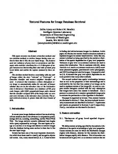
type. This model is denoted as uniform clique MRF model �68]. There are clearly problems related to the use of this model. Firstly, it is important that a signi�cant fraction of clique instances are uniform� otherwise most clique instances would have the potential � and the model would have little discriminatory power. It follows that the intensity value in an image must be quantized to very few levels. This can be seen in Derin and Cole �22] and Derin and Elliott �23] where at most four levels of quantization are used. This degree of quantization is likely to discard some of the texture feature information in the original texture. Secondly, the potential function does not take into account whether distinct intensity levels are close in value or not. This may lead to the fact that for distinct textures the clique instances will have identical patterns of uniformity and non-uniformity. In summary, uniform clique MRFs derive directly from the random �eld model of texture. However, practical considerations have forced unrealistic simpli�cations to be made. Wold-Based Representations. Picard and Liu �60] developed a new model based on the Wold decomposition for regular stationary stochastic processes in 2D images. If an image is assumed to be a homogeneous 2D discrete random �eld, then the 2D Wold-like decomposition is a sum of three mutually orthogonal components: a harmonic �eld, a generalized evanescent �eld, and a purely indeterministic �eld. These three components are illustrated in Fig. 3.4 by three textures, each of which is dominated by one of
3. Texture Features
61
these components. Qualitatively, these components appear as periodicity, directionality, and randomness, respectively.
Fig. 3.4 The Wold decomposition transforms textures into three orthogonal components: harmonic, evanescent, and random. The upper three textures illustrate these components� below each texture is shown its discrete Fourier transform (DFT) magnitude.
The motivation for choosing a Wold-based model, in addition to its signi�cance in random �eld theory, is its interesting relationship to independent psychophysical �ndings of perceptual similarity. Rao and Lhose �63] made a study where humans grouped patterns according to perceived similarity. The three most important similarity dimensions identi�ed in this study were repetitiveness, directionality, and complexity. These dimensions might be considered the perceptual equivalents of the harmonic, evanescent, and indeterministic components, respectively, in the Wold decomposition. Consider a homogeneous and regular random �eld fy(m n)j(m n) 2 Z 2 g. The 2D Wold decomposition allows the �eld to be decomposed into two mutually orthogonal components �30]:
y(m n) = v(m n) + w(m n) (3.4) where v(m n) is the deterministic component, and w(m n) is the indeterministic one. The deterministic component can be further decomposed into a mutually orthogonal harmonic component h(m n), and an evanescent component g(m n):
62
Sebe and Lew
v(m n) = h(m n) + g(m n):
(3.5)
In the frequency domain, the spectral distribution function (SDF) of
fy(m n)g can be uniquely represented by the SDFs of its component �elds:
Fy (� �) = Fv (� �) + Fw (� �) (3.6) where Fv (� �) = Fh (� �) + Fg (� �), and functions Fh (� �) and Fg (� �) cor-
respond to spectral singularities supported by point-like and line-like regions, respectively. A Wold-based model can be built by decomposing an image into its Wold components and modeling each of the components separately. Two decomposition methods have been proposed in the literature. The �rst is a maximum likelihood direct parameter estimation procedure, which provides parametric descriptions of image Wold components �31]. The authors reported that the algorithm can be computationally expensive, especially when the number of spectral peaks is large or the energy in the spectral peaks is not very high compared to that in the neighboring Fourier frequencies. Unfortunately, these situations often arise in natural images. The second method is a spectral decomposition procedure �29] which applies a global threshold to the image periodogram, and selects the Fourier frequencies with magnitude values larger than the threshold to be the harmonic or the evanescent components. Although this method is computationally e�cient, it is not robust enough for the large variety of natural texture patterns. The problem here is that the support region of an harmonic peak in a natural texture is usually not a point, but a small spread surrounding the central frequency. Therefore, two issues are essential for a decomposition scheme: locating the spectral peak central frequencies and determining the peak support regions. A new spectral decomposition-based approach which addresses these issues is presented in �50]. The algorithm decomposes an image by extracting its Fourier spectral peaks supported by point-like or line-like regions. After that, a spectral approach locates the peak central frequencies and estimates the peak support.
3.2.2 Non-Parametric PDF Methods The distinction between parametric and non-parametric methods re�ects the distinction made in statistics between parametric and non-parametric PDF modeling techniques. The methods described in this section also model the PDF of a pixel intensity as a function of the intensities of neighboring pixels. However, the methods described here use, in statistical parlance, nonparametric PDF models. Gray-Level Co-occurrence Matrices. Spatial gray-level co-occurrence estimates image properties related to second order statistics. Haralick �37] suggested the use of gray-level co-occurrence matrices (GLCM) which have become one of the most well-known and widely used texture features. The
3. Texture Features
63
G � G gray-level co-occurrence matrix Pd for a displacement vector d = (dx dy) is de�ned as follows. The entry (i j ) of Pd is the number of occurrences of the pair of gray-levels i and j which are a distance d apart. Formally, it is given as: Pd (i j ) = jf((r s) (t v)) : (t v) = (r + dx s + dy) I (r s) = i I (t v) = j gj where (r s), (t v) 2 N � N and j � j is the cardinality of a set. 1
1
2
2
2
1
1
2
2
2
1
3
3
3
3
3
4
3
3
4
1
2
3
4
1
2
2
1
0
3
2
0
4
0
0
4
4
3
0
0
5
2
4
4
4
0
0
0
4
a
b
Fig. 3.5 Gray-level co-occurrence matrix computation� a an image is quantized to four intensity levels, b the corresponding GLC matrix is computed with the o�set (dx dy) = (1 0).
An example is given in Fig. 3.5. In Fig. 3.5(a) there are boxed two pairs of pixels which have I (x y) = 1 and I (x + dx y + dy) = 2. The corresponding bin in the GLC matrix is emphasized in Fig. 3.5(b). Note that the co-occurrence matrix de�ned in this way is not symmetric. A symmetric variant can be computed using the formula: P = Pd + P;d . The cooccurrence matrix reveals certain properties about the spatial distribution of the gray-levels in the texture image. For example, if most of the entries in the co-occurrence matrix are concentrated along the diagonals, then the texture is coarse with respect to the displacement vector d. Haralick proposed a number of texture features that can be computed from the co-occurrence matrix. Some features are listed in Table 3.1. Here �x andP�y are the means and �Px and �y are the standard deviations of Pd (x) = j Pd (x j ) and Pd (y) = i Pd (i y ). The co-occurrence matrix features su�er from a number of di�culties. There is no well established method of selecting the displacement vector d and computing co-occurrence matrices for a lot of di�erent values of d is not feasible. Moreover, for a given d, a large number of features can be computed. This means that some sort of feature selection method must be
64
Sebe and Lew
Table 3.1 Some texture features extracted from gray-level co-occurrence matrices
Texture feature Energy Entropy Contrast Homogeneity Correlation
Formula 2 d( )
PP i
j
P
i j
; P P d ( ) log d ( ) P P ( ; )2 ( ) d P P d( ) i
P
j
i
i j
i
j
j
P
i
Pi Pj ( ; i
j
1+
P
P
i j
i j
i j
j;j i
j
x )(j ;�y )Pd (i j ) x y
�
� �
used to select the most relevant features. These methods have primarily been used in texture classi�cation tasks and not in segmentation tasks. Gray-Level Di�erence Methods. As noted by Weszka et al. �80], graylevel di�erence (GLD) methods strongly resemble GLC methods. The main di�erence is that, whereas the GLC method computes a matrix of intensity pairs, the GLD method computes a vector of intensity di�erences. This is equivalent to summing a GLC matrix along its diagonals. Formally, for any given displacement d = (dx dy), let Id (x y) = jI (x y); I (x + dx y + dy)j. Let pd be the probability density of Id (x y). If there are m gray-levels, this has the form of an m-dimensional vector whose ith component is the probability that Id (x y) will have value i. If the image I is discrete, it is easy to compute pd by counting the number of times each value of Id (x y) occurs. Similar features as in Table 3.1 can be computed. Texture Spectrum Methods. All methods described above model texture as a random �eld. They model the intensity of a pixel as a stochastic function of the intensities of neighboring pixels. However, the space of all possible intensity patterns in a neighborhood is huge. For example, if a 5 � 5 neighborhood is considered (excluding the central pixel), the PDF is a function in a 24-dimensional space. GMRF and GLC methods rely on assumptions that reduce the complexity of the PDF model. GRMF methods estimate the intensity as a function of all the neighboring pixels but assume that the distribution is Gaussian and is centered on a linear function of the neighboring intensities. The GLC method uses a histogram model� this requires the space of intensities to be partitioned into histogram bins. The partitioning is only sensitive to second order interactions but not to higher order interactions. Texture spectrum methods use PDF models which are sensitive to high order interactions. Typically, these methods use a histogram model in which the partitioning of the intensity space is sensitive to high order interactions between pixels. This sensitivity is made feasible by quantizing the intensity
3. Texture Features
65
values to a small number of levels, which considerably reduces the size of the space. The largest number of levels used is four but two levels, or thresholding, is more common. Ojala et al. �56] proposed a texture unit represented by eight elements, each of which has two possible values f0 1g obtained from a neighborhood of 3 � 3 pixels. These texture units are called local binary patterns (LBP) and their occurrence of distribution over a region forms the texture spectrum. The LBP is computed by thresholding each of the noncenter pixels by the value of the center pixel, resulting in 256 binary patterns. The LBP method is a gray-scale invariant and can be easily combined with a simple contrast measure by computing for each neighborhood the di�erence of the average gray-level of those pixels which after thresholding have the value 1, and those which have the value 0, respectively. The algorithm is detailed below. For each 3 � 3 neighborhood, consider Pi the intensities of the component pixels with P0 the intensity of the center pixel. Then,
(
by the value of the center pixel: 0 = 01 ifotherwise0 P8 0 . 2. Count the number of resulting non-zero pixels: = 1. Threshold pixels
Pi
n
n
3. Calculate the local binary pattern: 4. Calculate the local contrast: 80 < 8 8 = :1 P 0 ; 1 P (1 ; 0 ) 8; C
n
i=1
Pi Pi
Pi < P
Pi
n
LBP
i=1
P8 0 2 ;1 .
i=1
Pi
Pi
i
if = 0 or = 8 otherwise. n
Pi Pi
i=1
=
:
n
A numerical example is given in Fig. 3.6. Thresholded
Example 6
5
2
1
0
1
0
0
0
8
1111 0000 0000 1111 0000 1111 0000 1111 0000 1111 0000 1111 0000 1111 0000 1111
0
1
32
0
128
0
7
6
1
1
1111 0000 0000 1111 0000 1111 0000 1111 0000 1111 0000 1111 1111 0000 1111 0000
9
3
7
1
0
LBP=1+8+32+128=169
Weights
C=(6+7+9+7)/4-(5+2+1+3)/4=4.5
Fig. 3.6 Computation of local binary pattern (LBP) and contrast measure (C).
66
Sebe and Lew
The LBP method is similar to the methods described by Wang and He �78] and by Read et al. �64]. These methods generate more distinct texture units than LBP. Wang and He �78] quantize to three intensity levels, giving 38 or 6561 distinct texture units. Read et al. �64] quantize the image to four intensity levels, but use only a 3 � 2 neighborhood. This gives 46 or 4096 distinct texture units. Another class of texture spectrum methods consists of N -tuple methods �2, 6]. Whereas the texture units in the methods described above use all the pixels in a small neighborhood, the N -tuple methods use a subset of pixels from a larger neighborhood. Typically, subsets of 6 to 10 pixels are used from a 6 � 6 to a 10 � 10 neighborhood. These subsets are selected randomly� a typical N -tuple memory algorithm might have 30 N -tuple units, each of which has a distinct random subset of pixels in the neighborhood. The texture unit histogram and texture class information are computed independently for each N -tuple unit. Texture class information from each N -tuple unit is combined to give the texture class information of the N -tuple memory. In summary, texture spectrum methods are sensitive to high order interactions between pixels. This is made feasible by reducing the size of the space of intensities by quantization. Even in this reduced space, only a limited number of pixels, typically less than 10, contribute to the feature vector that characterizes the texture.
3.2.3 Harmonic Methods The main methods in this category are the Fourier power spectrum and autocorrelation methods. These two methods are intimately related, since the autocorrelation function and the power spectral function are Fourier transforms of each other �38]. Harmonic methods model a texture as a summation of waveforms so they assume that intensity is a strongly periodic function of the spatial coordinates. Autocorrelation Features. An important property of many textures is the repetitive nature of the placement of texture elements in the image. The autocorrelation function of an image can be used to assess the amount of regularity as well as the �neness/coarseness of the texture present in the image. Formally, the autocorrelation function of an image I is de�ned as follows: N P N P I (u v)I (u + x v + y) : (x y) = u=0 v=0 P N P N 2 I (u v)
(3.7)
u=0 v=0
Examples of autocorrelation functions for some Brodatz textures are shown in Fig. 3.7. The autocorrelation functions of non-periodic textures are
3. Texture Features
67
dominated by a single peak. The breadth and elongation of the peak is determined by the coarseness and directionality of the texture. In a �ne-grained texture, as in Fig. 3.7(a), the autocorrelation function will decrease rapidly, generating a sharp peak. On the other hand, in a coarse-grained texture, as in Fig. 3.7(b), the autocorrelation function will decrease more slowly, generating a broader peak. A directional texture (Fig. 3.7(c)) will generate an elongated peak. For regular textures (Fig. 3.7(d)) the autocorrelation function will exhibit peaks and valleys.
a
b
c
d
Fig. 3.7 Autocorrelation functions computed for four Brodatz textures. The discriminatory power of the autocorrelation methods have been compared with other methods, empirically by Weszka et al. �80], and theoretically by Conners and Harlow �17]. Both studies �nd that the autocorrelation methods are less powerful discriminators than GLC methods. Weszka suggests that this is due to the inappropriateness of the texture model: \the textures ... may be more appropriately modeled statistically in the space domain (e.g., as random �elds with speci�ed autocorrelation), rather than as a sum of sinusoids." Fourier Domain Features. The frequency analysis of the textured image is best done in the Fourier domain. As the psychophysical results indicated, the human visual system analyzes the textured images by decomposing the image into its frequency and orientation components �10]. The multiple channels tuned to di�erent frequencies are also referred to as multi-resolution processing in the literature. Similar to the behavior of the autocorrelation function is the behavior of the distribution of energy in the power spectrum. Early approaches using spectral features divided the frequency domain into rings (for frequency content) and wedges (for orientation content). The frequency domain is thus divided into regions and the total energy in each of these regions is computed as a texture feature. For example the energy computed in a circular band is a feature indicating coarseness/�neness:
68
Sebe and Lew
fr �r = 1
Z 2� Z r
2
2
r1
0
jF (u v)j2 drd�
(3.8)
and the energy computed in each wedge is a feature indicating directionality:
f� �� = 1
Z� Z1
2
p
2
�1
0
jF (u v)j2 drd�
(3.9)
where r = u2 + v2 and � = arctan(v=u). In summary, harmonic methods are based on a model of texture consisted of sums of sinusoidal waveforms which extend over large regions. However, the modern literature, supported by empirical results, favors modeling texture as a local phenomenon, rather than a phenomenon with long range interactions.
3.2.4 Primitive Methods This section reviews primitive methods including textural \edgeness," convolution, and mathematical morphology methods. Many of the texture primitives used in these methods have a speci�c scale and orientation. For example, lines and edges have a well-de�ned orientation, and the scale of a line is determined by its width. As seen before, harmonic methods also measure scale (frequency of wavelength) and orientation speci�c features. In particular, there is a strong relationship between primitive methods such as Gabor convolutions and Fourier transforms� essentially, a Gabor convolution is a spatially localized Fourier transform �20]. However, the distinction between these methods is straightforward: primitive methods measure spatially local features, whereas harmonic methods measure spatially dispersed features. Primitive methods are also related to structural texture methods. Both methods model textures as being composed of primitives. However, structural methods tend to have one arbitrarily complex primitive, whereas primitive methods model texture as composed of many, simple primitives. Moreover, the relative placement of primitives is important in structural methods but plays no role in primitive methods. Early Primitive Methods. Spatial domain �lters are the most direct way to capture image texture properties. Earlier attempts at de�ning such methods concentrated on measuring the edge density per unit area. Fine textures tend to have a higher density of edges per unit area than coarser textures. The measurement of edgeness is usually computed by simple edge masks such as Robert's operator or the Laplacian operator. The edgeness measure can be computed over an image area by computing a magnitude from the response of Robert's mask or from the response of the Laplacian mask. Hsu �40] takes a di�erent approach. He measures the pixel-wise intensity di�erence between the actual neighborhood and a uniform intensity� this distance is used as a measure of the density of edges.
3. Texture Features
69
Laws �48] describes a set of convolution �lters which respond to edges, extrema, and segments of high frequency waveforms. A two-step procedure is proposed. In the �rst step, an image is convolved with a mask, and in the second the local variance is computed over a moving window. The proposed masks are small, separable, and simple and can be regarded as low cost, i.e., computationally inexpensive, Gabor functions. Malik and Perona �53] proposed a spatial �ltering to model the preattentive texture perception in the human visual system. They propose three stages: (1) convolution of the image with a bank of even-symmetric �lters followed by a half-wave recti�cation, (2) inhibition of spurious responses in a localized area, and (3) detection of boundaries between the di�erent textures. The even-symmetric �lters used by them consist of di�erences of o�set Gaussian functions. The half-wave recti�cation and inhibition are methods of introducing a non-linearity into the computation of texture features. This non-linearity is needed in order to discriminate texture pairs with identical mean brightness and identical second order statistics. The texture boundary detection is done by a straightforward edge detection method applied to the feature images obtained from stage (2). This method works on a variety of texture examples and is able to discriminate natural as well as synthetic textures with carefully controlled properties. Gabor and Wavelet Models. The Fourier transform is an analysis of the global frequency content in the signal. Many applications require the analysis to be localized in the spatial domain. This is usually handled by introducing spatial dependency into the Fourier analysis. The classical way of doing this is through what is called the window Fourier transform. Considering a onedimensional signal f (x), the window Fourier transform is de�ned as:
Fw (u �) =
Z1
;1
f (x)w(x ; �)e;j2�ux dx:
(3.10)
When the window function w(x) is Gaussian, the transform becomes a Gabor transform. The limits of the resolution in the time and frequency domain of the window Fourier transform are determined by the time{bandwidth product or the Heisenberg uncertainty inequality given by t u � 41� . Once a window is chosen for the window Fourier transform, the time{frequency resolution is �xed over the entire time{frequency plane. To overcome the resolution limitation of the window Fourier transform, one lets the t and u vary in the time{frequency domain. Intuitively, the time resolution must increase as the central frequency of the analyzing �lter is increased. That is, the relative bandwidth is kept constant in a logarithmic scale. This is accomplished by using a window whose width changes as the frequency changes. Recall that when a function f (t) is scaled in time by a, which is expressed as f (at), the function is contracted if a > 1 and it is expanded when a < 1. Using this fact, the wavelet transform can be written as:
70
Sebe and Lew
Z 1 Wf�a (u �) = pa
1
;1
f (t)h
�t ; � a
dt:
(3.11)
Setting in Eq. 3.11,
h(t) = w(t)e;j2�ut
(3.12)
we obtain the wavelet model for texture analysis. Usually the scaling factor will be based on the frequency of the �lter. Daugman �19] proposed the use of Gabor �lters in the modeling of receptive �elds of simple cells in the visual cortex of some mammals. The proposal to use the Gabor �lters in texture analysis was made by Turner �74] and Clark and Bovik �16]. Gabor �lters produce frequency decompositions that achieve the theoretical lower bound of the uncertainty principle �20]. They attain maximum joint resolution in space and frequency bounded by the relations x u � 41� and y v � 41� , where � x y] gives the resolution in space and � u v] gives the resolution in frequency. A two-dimensional Gabor function consists of a sinusoidal plane wave of a certain frequency and orientation modulated by a Gaussian envelope. It is given by:
� �
2 2 g(x y) = exp ; 21 �x2 + �y 2 cos(2�u0 (x cos � + y sin �)) (3.13) x y where u0 and � are the frequency and phase of the sinusoidal wave, respectively. The values �x and �y are the sizes of the Gaussian envelope in the x and y directions, respectively. The Gabor function at an arbitrary orientation �0 can be obtained from Eq. 3.13 by a rigid rotation of the xy plane by �0 .
The Gabor �lter is a frequency and orientation selective �lter. This can be seen from the Fourier domain analysis of the function. When the phase � is 0, the Fourier transform of the resulting even-symmetric Gabor function g(x y) is given by:
� � � � � 2 2 2 2 G(u v)= A exp ; 12 (u ;�2u0) + �v 2 + exp ; 12 (u +�2u0 ) + �v 2 u v u v where �u = 1=(2��x), �v = 1=(2��y ) and A = ��x �y . This function is
real-valued and has two lobes in the frequency domain, one centered around
u0 , and another centered around ;u0 . For a Gabor �lter of a particular
orientation, the lobes in the frequency domain are also appropriately rotated. The Gabor �lter masks can be considered as orientation and scale tunable edge and line detectors. The statistics of these microfeatures in a given region can be used to characterize the underlying texture information. A class of such self-similar functions referred to as Gabor wavelets is discussed by Ma and Manjunath �51]. This self-similar �lter dictionary can be obtained by appropriate dilations and rotations of g(x y) through the generating function,
3. Texture Features
gmn (x y) = a;m g(x0 y0 ) m = 0 1 : : : S ; 1
71
(3.14)
x0 = a;m (x cos � + y sin �) y0 = a;m (;x sin � + y cos �) where � = n�=K , K the number of orientations, S the number of scales in the multiresolution decomposition, and a = (Uh =Ul );1=(S;1) with Ul and Uh
the lower and the upper center frequencies of interest, respectively. An alternative to gain in the trade-o� between space and frequency resolution without using Gabor functions is using a wavelet �lter bank. The wavelet �lter bank produces octave bandwidth segmentation in frequency. It allows simultaneously for high spatial resolutions at high frequencies and high frequency resolution at low frequencies. Furthermore, the wavelet tiling is supported by evidence that visual spatial-frequency receptors are spaced at octave distances �21]. A quadrature mirror �lter (QMF) bank was used for texture classi�cation by Kundu and Chen �47]. A two-band QMF bank utilizes orthogonal analysis �lters to decompose data into low-pass and highpass frequency bands. Applying the �lters recursively to the lower frequency bands produces wavelet decomposition as illustrated in Fig. 3.8. µ0 σ0
Wavelet Transform
µ3σ3 µ6σ6 µ7σ7 µ9σ9 µ8σ8
µ4σ4 µ5σ5
µ1 σ1
µ2 σ2
Feature Vector µ0σ0 ,..., µnσn
Fig. 3.8 Texture classi�er for Brodatz textures samples using QMF-wavelet based features.
The wavelet transformation involves �ltering and subsampling. A compact representation needs to be derived in the transform domain for classi�cation and retrieval. The mean and the variance of the energy distribution of the transform coe�cients for each subband at each decomposition level are used to construct the feature vector (Fig. 3.8) �67]. Let the image subband be Wn (x y), with n denoting the speci�c subband. Note that in the case of Gabor wavelet transform (GWT) there are two indexes m and n with m indicating a certain scale and n a certain orientation �51]. The resulting feature vector is f = (�n �n ) with,
Z
�n = jWn (x y)jdx dy �n =
sZ
(jWn (x y)j ; �n )2 dx dy:
(3.15) (3.16)
72
Sebe and Lew
Consider two image patterns i and j and let f (i) and f (j) represent the corresponding feature vectors. The distance between the two patterns in the features space is:
d(f (i)
X f (j ) ) = n
�� (i) (j) �� �� (i) (j) ��! �� �n ; �n ��+ �� �n ; �n �� � �(�n ) � � �(�n ) �
(3.17)
where �(�n ) and �(�n ) are the standard deviations of the respective features over the entire database. Jain and Farrokhina �41] used a version of the Gabor transform in which window sizes for computing the Gabor �lters are selected according to the central frequencies of the �lters. They use a bank of Gabor �lters at multiple scales and orientations to obtain �ltered images. Each �ltered image is passed through a sigmoidal nonlinearity. The texture feature for each pixel is computed as the absolute average deviation of the transform values of the �ltered images from the mean with a window W of size M � M . The �ltered images have zero mean, therefore, the ith texture feature image ei (x y) is given by the equation: X e (x y) = 1 j�(r (a b))j (3.18) i
M 2 (a�b)2W
i
where ri (x y) is the �ltered image for the ith �lter and �(t) is the nonlinearity having the form of tanh(�t), where the choice of � is determined empirically. Mathematical Morphology. Haralick �38] reviews mathematical morphology methods. These methods generate transformed images by erosion and dilation with structural elements. These structural elements correspond to texture primitives. For example, consider a binary image with pixel values on and o . A new image can be formed in which a pixel is on if the corresponding pixel and all pixels within a certain radius, in the original image are on. This transformation is an erosion with a circular structural element. The number of on pixels in the transformed image will be a function of the texture in the original image and of the structural element. For example, consider a strongly directional texture, such as a striped image, and an elongated structural element. If the structural element is perpendicular to the stripes, there will be very few on pixels in the transformed image. However, if the structural element is elongated in the same direction as the stripes, most of the on pixels in the original image will be also on in the transformed image. Thus, the �rst order properties of the transformed image re�ect the density, in the original image, of the texture primitive corresponding to the structural element.
3.2.5 Fractal Methods Fractal methods are distinguished from other methods by explicitly encoding the scaling behavior of the texture. Fractals are useful in modeling di�erent
3. Texture Features
73
properties of natural surfaces like roughness and self-similarity at di�erent scales. Self-similarity across scales in fractal geometry is a crucial concept. A deterministic fractal is de�ned using this concept of self-similarity as follows. Given a bounded set A in an Euclidean n-space, the set A is said to be selfsimilar when A is the union of N distinct (non-overlapping) copies of itself, each of which has been scaled down by a ratio of r. The fractal dimension D is related to the number N and the ratio r as follows: log N : (3.19) D = log(1 =r) The fractal dimension gives a measure of the roughness of a surface. Intuitively, the larger the fractal dimension is, the rougher the texture is. Pentland �57] argued and gave evidence that images of most natural surfaces can be modeled as spatially isotropic fractals. However, most natural texture surfaces are not deterministic but have a statistical variation. This makes the computation of fractal dimension more di�cult. There are a number of methods proposed for estimating the fractal dimension. One method is the estimation of the box dimension �46]. Given a bounded set A in an Euclidean n-space, consider boxes of size Lmax on a side which cover the set A. A scaled down version of the set A by ratio r will result in N = 1=rD similar sets. This new set can be covered by boxes of size L = rLmax. The number of such boxes is related to the fractal dimension:
� D N (L) = r1D = Lmax : L
(3.20)
The fractal dimension is estimated from Eq. 3.20 by the following procedure. For a given L, divide the n-space into a grid of boxes of size L and count the number of boxes covering A. Repeat this procedure for di�erent values of L. The fractal dimension D can be estimated from the slope of the line: ln(N (L)) = ;D ln(L) + D ln(Lmax ):
(3.21)
Another method for estimating the fractal dimension was proposed by Voss �77]. Let P (m L) be the probability that there are m points within a box of side length L centered at an arbitrary point of a surface A. Let M be the total number of points in the image. When one overlays the image with boxes of side length L, then the quantity (M=m)P (m L) is the expected number of boxes with m points inside. The expected total number of boxes needed to cover the whole image is:
E �N (L)] = M
N X
1 P (m L): m m=1
(3.22)
74
Sebe and Lew
The expected value of N (L) is proportional to L;D and thus can be used to estimate the fractal dimension. Super and Bovik �69] proposed a method based on Gabor �lters to estimate the fractal dimension in textured images. The fractal dimension alone is not su�cient to completely characterize a texture. It has been shown �46] that there may be perceptually very different textures that have very similar fractal dimensions. Therefore, another measure called lacunarity �46, 77] has been suggested in order to capture the textural property that will distinguish between such textures. Lacunarity is de�ned as follows:
�=E
"�
2 #
M E �M ] ; 1
(3.23)
where M is the mass of the fractal set and E �M ] is its expected value. Lacunarity measures the discrepancy between the actual mass and the expected value of the mass: lacunarity is small when the texture is �ne and it is large when the texture is coarse. The mass of the fractal set is related to the length L by the power law: M (L) = KLD . Voss �77] computedPthe lacunarity from the probability P distribution P (m L). Let M (L) = Nm=1 mP (m L) and M 2 (L) = Nm=1 m2 P (m L). Then the lacunarity � is given by: 2 ) ; (M (L))2 �(L) = M (L(M : (L))2
(3.24)
For fractal textures, the fractal dimension is a theoretically sound feature. However, many real-world textures are not fractal in the sense of obeying the self-similarity law. Any texture with sharp peaks in its power spectrum does not obey the self-similarity law.
3.2.6 Line Methods Line methods are distinguished by measuring features from one-dimensional (though possibly curved) subsets of texture. These methods are computationally cheap. They were among the earliest texture methods being attractive in those times possibly because of their computational cheapness. These methods are not derived from the de�nition of texture as a locally structured two-dimensional homogeneous random �eld. Barba and Ronsin �3], performed a curvilinear integration of the gray-level signal along some half scan lines starting from each pixel and in di�erent orientations. The scan line ends when the integration reaches a preset value. The measure of texture is then given by the vector of displacements along the lines of di�erent orientations.
3. Texture Features
75
Another line method is the gray-level run length method �33] which is based on computing the number of gray-level runs of various lengths. A graylevel run is a set of linearly adjacent image pixels having the same gray value. The length of the run is the number of pixels within the run. The element r0 (i j j�) of the gray-level run length matrix speci�es the number of times an image contains a run of length j for gray-level i in the angle � direction. These matrices usually are calculated for several values of �.
3.2.7 Structural Methods The structural models of texture assume that textures are composed of texture primitives. They consider that the texture is produced by the placement of the primitives according to certain placement rules. Structural methods are related to primitive methods because both model textures as being composed of primitives. However, structural methods tend to have one arbitrarily complex primitive, whereas primitive methods model texture as composed of many, simple primitives. Moreover, the relative placement of primitives is important in structural methods but plays no role in primitive methods. Structural-based algorithms are in general limited in power unless one is dealing with very regular textures. There are a number of ways to extract texture elements in images. Usually texture elements consist of regions in the image with uniform gray-levels (blobs or mosaics). Blob methods segment the image into small regions. In the mosaic algorithms the regions completely cover the image, forming a mosaiclike tessellation of the image �38, 72]. In some blob methods, the regions do not completely cover the image, forming a foreground of non-touching blobs. A blob or mosaic method models the image as composed of one simple but variable primitive� the measured features model the variations of the primitive found in the image. Voorhees �76] and Chen et al. �15] describe methods in which features are extracted from non-contiguous blobs. Voorhees convolves the image with a center surround �lter and thresholds the resulting convolution image slightly below zero. This gives an image consisting of many foreground blobs corresponding to dark patches in the original image. He characterizes a texture by the contrast, orientation, width, length, area, and area density of blobs within the texture. Chen et al. threshold the original image at several different intensities generating a separate binary image for each threshold. In these binary images contiguous pixels above the intensity threshold form bright blobs� likewise, contiguous pixels below the intensity threshold form dark blobs. The average area and irregularity of these blobs are measured for each intensity threshold, giving features which measure the granularity and elongation of the texture. Tuceryan and Jain �72] proposed the extraction of texture tokens by using the properties of the Voronoi tessellation of the given image. Voronoi tessellation has been proposed because of its desirable properties in de�ning local
76
Sebe and Lew
spatial neighborhoods and because the local spatial distributions of tokens are re�ected in the shapes of the Voronoi polygons. Firstly, texture tokens are extracted and then the tessellation is constructed. Tokens can be as simple as points of high gradient in the image or complex structures such as line segments or closed boundaries. Features of each Voronoi cell are extracted and tokens with similar features are grouped to construct uniform texture regions. Moments of the area of the Voronoi polygons serve as a useful set of features that re�ect both the spatial distribution and shapes of the tokens in the textured image. Zucker �81] has proposed a method in which he regards the observable textures (real textures) as distorted versions of ideal textures. The placement rule is de�ned for the ideal texture by a graph that is isomorphic to a regular or semiregular tessellation. These graphs are then transformed to generate the observable texture. Which of the regular tessellations is used as the placement rule is inferred from the observable texture. This is done by computing a two-dimensional histogram of the relative positions of the detected texture tokens. Another approach to modeling texture by structural means is described by Fu �32]. Here the texture primitives can be as simple as a single pixel that can take a gray value, but is usually a collection of pixels. The placement rule is de�ned by a tree grammar. A texture is then viewed as a string in the language de�ned by the grammar whose terminal symbols are the texture primitives. An advantage of these methods is that they can be used for texture generation as well as texture analysis. The patterns generated by the tree grammars could also be regarded as ideal textures in Zucker's model �81].
3.3 Texture in Content-Based Retrieval With content-based techniques, the important visual features of images are described mathematically using feature sets that are derived from the digital data. If chosen properly, the feature sets may coincide well with intuitive human notions of visual content while providing e�ective mathematical discrimination. Furthermore, the features may be extracted automatically without requiring human assistance. This approach allows the database to be indexed using the discriminating features that characterize visual content, and to be searched using visual keys. A content-based search of the database proceeds by �nding the items most mathematically and visually similar to the search key. Interest in visual texture was triggered by the phenomenon of texture discrimination which occurs when a shape is de�ned purely by its texture, with no associated change in color or brightness: color alone cannot distinguish between tigers and cheetahs! This phenomenon gives clear justi�cation for texture features to be used in content-based retrieval together with color and shape. Several systems have been developed to search through image
3. Texture Features
77
databases using texture, color, and shape attributes (QBIC �12], Photobook �58], Chabot �55], VisualSEEk �66], etc.). Although, in these systems texture features are used in combination with color and shape features, texture alone can also be used for content-based retrieval. In practice, there are two di�erent approaches in which texture is used as main feature for content-based retrieval. In the �rst approach, texture features are extracted from the images and then are used for �nding similar images in the database �34, 52, 67]. Texture queries can be formulated in a similar manner to color queries, by selecting examples of desired textures from a palette, or by supplying an example query image. The system then retrieves images with texture measures most similar in value to the query. The systems using this approach may use already segmented textures as in the applications with Brodatz database �59], or they �rst have a segmentation stage after which the extracted features in di�erent regions are used as queries �52]. The segmentation algorithm used in this case may be crucial for the content-based retrieval. In the second approach, texture is used for annotating the image �61]. Vision-based annotation assists the user in attaching descriptions to large sets of images and video. If a user labels a piece of an image as \water," a texture model can be used to propagate this label to other visually similar regions. What distinguishes image search for database-related applications from traditional pattern classi�cation methods is the fact that there is a human in the loop (the user), and in general there is a need to retrieve more than just the best match. In typical applications, a number of top matches with rank-ordered similarities to the query pattern will be retrieved. Comparison in the feature space should preserve visual similarities between patterns.
3.3.1 Texture Segmentation As mentioned before, texture segmentation algorithms may be critical for the success of content-based retrieval. The segmentation process may be the �rst step in processing the user query. The segmentation is a di�cult problem because one usually does not know a priori what types of textures exist in an image, how many di�erent textures there are, and what regions have which texture. Generally speaking, one does not need to know which textures are present in the image in order to do segmentation. All that is needed is a way to tell that two textures, usually present in adjacent regions, are di�erent. The performance of a segmentation method strongly depends on the quality of input features, i.e., the noise within homogeneous regions and the amplitude separation between them. In general, a segmentation method is judged according to its capacity to eliminate very small subregions within more substantial ones, in combination with its accuracy in locating region boundaries. These capabilities, which are strongly connected to an analysis of the local image content, distinguish segmentation from supervised pixel classi�cation,
78
Sebe and Lew
where feature statistics are gathered over homogeneous training areas and pixels are classi�ed without further using any local image information. There are two general approaches to performing texture segmentation: region-based approaches and boundary-based approaches. In a region-based approach �52], one tries to identify regions in the image which have a uniform texture. Pixels or small local regions are merged based on the similarity of some texture property. The regions having di�erent textures are then considered to be segmented regions. The advantage of this method is that the boundaries of regions are always closed and therefore, the regions with di�erent textures are always well separated. However, in general, one has to specify the number of distinct textures present in the image in advance. Additionally, thresholds on similarity values are needed. The boundary-based approaches �72, 76] are based upon the detection of di�erences in texture in adjacent regions. Here, one does not need to know the number of textured regions in the image in advance. However, the boundaries may not be closed and two regions with di�erent textures are not identi�ed as separate closed regions. Du Buf et al. �27] studied and compared the performance of various texture segmentation techniques and their ability to localize the boundaries. Tuceryan and Jain �72] use the texture features computed from the Voronoi polygons in order to compare the textures in adjacent windows. The comparison is done using a Kolmogorov{Smirno� test. A probabilistic relaxation labeling, which enforces border smoothness is used to remove isolated edge pixels and �ll boundary gaps. Voorhees and Poggio �76] extract blobs and elongated structures from images (they suggest that these correspond to Julesz's textons �44]). The texture properties are based on blob characteristics such as their sizes, orientations, etc. They then decide whether the two sides of a pixel have the same texture using a statistical test called maximum frequency di�erence (MFD). The pixels where this statistic is su�ciently large are considered to be boundaries between di�erent textures. A \blobworld" approach is used by Carson et al. �11]. In order to segment an image, the joint distribution of the color, texture, and position features of each pixel in the image is modeled. The expectation-maximization (EM) algorithm is used to �t a mixture of Gaussians to the data� the resulting pixel-cluster memberships provide the segmentation of the image. After the image is segmented into regions, a description of each region's color, texture, and spatial characteristics is produced. Ma and Manjunath �52] propose a segmentation scheme which is appropriate for large images (large aerial photographs) and database retrieval applications. The proposed scheme utilizes Gabor texture features extracted from the image tiles and performs a coarse image segmentation based on local texture gradients. For such image retrieval applications accurate pixel level segmentation is often not necessary although the proposed segmentation method can achieve pixel-level accuracy. In the �rst stage, using the feature
3. Texture Features
79
vectors, a local texture gradient is computed between each image tile and its surrounding eight neighbors. The dominant �ow direction is identi�ed in a competitive manner which is similar to a winner-takes-all representation. This is called texture edge �ow as the gradient information is propagated to neighboring pixels (or tiles). The texture edge �ow contains information about the (spatial) direction and energy of the local texture boundary. The next stage is the texture edge �ow propagation. Following the orientation competition, the local texture edge �ow is propagated to its neighbors, if they have the same directional preference. The �ow continues until it encounters an opposite �ow. This helps to localize the precise positions of the boundaries and concentrate the edge energies towards pixels where the image boundaries might exist. After the propagation reaches a stable state, the �nal texture edge �ow energy is used for boundary detection. This is done by turning on the edge signals between two neighboring image tiles, if their �nal texture edge �ow points in opposite directions. The texture energy is then de�ned to be the summation of texture edge �ow energies in the two neighboring image tiles. This stage results in many discontinuous image boundaries. In the �nal stage, these boundaries are connected to form an initial set of image regions. At the end, a conservative region merging algorithm is used to group similar neighboring regions.
3.3.2 Texture Classi cation and Indexing Texture classi�cation involves deciding what texture category an observed image belongs to. In order to accomplish this, one needs to have a priori knowledge of the classes to be recognized. Once this knowledge is available and the texture features are extracted, the pattern classi�cation techniques can be used in order to do the classi�cation. Examples where texture classi�cation was applied as the appropriate texture processing method include the classi�cation of regions in satellite images into categories of land use �37]. A recent extension of the technique is the texture thesaurus developed by Ma and Manjunath �52], which retrieves textured regions in images on the basis of similarity to automatically derived codewords (thesaurus) representing important classes of texture within the collection. This approach can be visualized as an image counterpart of the traditional thesaurus for text search. It creates the information links among the stored image data based on a collection of codewords and sample patterns obtained from the training set. Similar to parsing text documents using a dictionary or thesaurus, the information within images can be classi�ed and indexed via the use of the texture thesaurus. The design of the thesaurus has two stages. The �rst stage uses a learning similarity algorithm to combine the human perceptual similarity with the low level feature vector information, and the second stage utilizes a hierarchical vector quantization technique to construct the codewords. The proposed texture thesaurus is domain dependent and can be designed to meet the particular need of a speci�c image data
80
Sebe and Lew
type by exploring the training data. It also provides an e�cient indexing tree while maintaining or even improving the retrieval performance in terms of human perception. Furthermore, the visual codeword representation in the thesaurus can be used as information samples to help users browse through the database. A collection of visual thesauri for browsing large collections of geographic images is also proposed by Ramsey et al. �62]. Each texture region of an image is mapped to an output node in a self-organizing map (SOM) representing a unique cluster of similar textures. The output node number can be treated as an index for the image texture region and can be used to compute co-occurrence with other texture types (i.e., textures mapped to other output nodes). Then, users can browse the visual thesaurus and �nd a texture to start their query. A list of other classes of textures frequently co-occurring with the speci�ed one is displayed in decreasing frequency order. From this list the user can re�ne the queries by selecting other textures they feel are relevant to their search.
3.3.3 Texture for Annotation Traditionally, access to multimedia libraries has been in the form of text annotation { titles, authors, captions, and descriptive labels. Text provides a natural means of summarizing massive quantities of information. Text keywords consume little space and provide fast access into large amounts of data. When the data is text, it can be summarized using sophisticated computer programs based on natural language processing and arti�cial intelligence. When the data is not text but is for example image, then generating labels is considerably more di�cult. Of course, some access to pictures is best achieved without text { for example, the user may wish to \�nd another image like this." In this case, a signal is compared to another signal and conversion to text is not required. However, annotation is both important for preparing multimedia digital libraries for query and retrieval, and useful for adding personal notes to the user's online collection. Tools that help annotate multimedia database need to be able to \see" as the human \sees" { so that if the human says \label this stu� grass" the computer will not only label that stu� but also �nd other grass that \looks the same" and label it too. Texture features, although low-level, play an important role in the high-level perception of visual scenes enabling the distinction of regions like \water" from \grass" or \buildings" from \sky." Such features alone do not solve the complete annotation problem but they are a key component of the solution. Picard and Minka �61] proposed a system to help generate descriptions for annotating image and video. They noticed that a single texture model is not su�cient to reliably match human perception of similarity in pictures. Rather than using one model, the proposed system knows several texture models and is equipped with the ability to choose the one which \best explains" the regions selected by the user for annotating. If none of these models su�ces, then the system creates new explanations by combining models. Determining
3. Texture Features
81
which model gives the best features for measuring similarity is hampered by the fact that the users are �ckle. People are nonlinear time-varying systems when it comes to predicting their behavior. A user may label the same scene di�erently, and expect di�erent regions to be recognized as similar when his or her goals change. In the system, the user can browse through a database of scenes. He or she can select patches from one or more images as \positive examples" for a label. The system then propagates the label to new regions in the database that it thinks should also have the same label. The user can immediately view the results and can remove falsely labeled patches by selecting them to be \negative examples" for the label. The user can continue to add positive or negative examples for the same label or di�erent labels. The system responds di�erently depending upon which patches are selected as positive or negative examples.
3.4 Summary Texture is the term used to characterize the surface of a given object or phenomenon and it is undoubtedly one of the main features used in image processing and pattern recognition. In an image, texture is one of the visual characteristics that identi�es a segment as belonging to a certain class. We recognize many parts of the image by texture rather than by shape, e.g., fur, hair, etc. If the texture belongs to a class that has a particular physical interpretation such as grass, hair, water, or sand, then it may be regarded as a \natural" texture. On the other hand, a texture may belong to a class identi�ed by arti�cial visual characteristics that have a concise mathematical interpretation. Despite its ubiquity, a formal de�nition of texture remains elusive. In the literature, various textural properties are often used to serve as the de�nition of texture, or more precisely to constrain the domain of problems. Some researchers formally de�ne texture by describing it in terms of the human visual system, whereas others are completely driven in de�ning texture by the application in which this de�nition is used. Identifying the perceived qualities of texture in an image is an important �rst step toward building mathematical models for texture. The intensity variations in an image which characterize texture are generally due to some underlying physical variations in the scene (e.g., waves in water). Modeling this physical variation is very di�cult, so texture is usually characterized by the two-dimensional variations in the intensities present in the image. Various methods of texture representation were presented. The literature distinguishes between stochastic/statistical and structural methods for texture. The use of statistical features is one of the early methods proposed in the machine vision literature. These methods are based on the spatial distribution of gray values in the image. In a stochastic approach, a texture is assumed to be the realization of a stochastic process which is governed by some parameters. Analysis is performed by de�ning a model and estimating the parameters so
82
Sebe and Lew
that the stochastic process can be reproduced from the model and associated parameters. In a structural approach a texture is viewed as a two-dimensional pattern consisting of a set of primitives or subpatterns which are arranged according to certain placement rules. Texture processing has been successfully applied in content-based retrieval. In practice, there are two di�erent approaches in which texture is used as main feature for content-based retrieval. In the �rst approach, an image can be considered as a mosaic of di�erent texture regions, and the image features associated with these regions can be used for search and retrieval. A typical query could be a region of interest provided by the user (e.g., a vegetation patch in a satellite image). This approach may involve an additional segmentation step which will identify the texture regions. In the second approach, texture is used for annotating the image. Here, vision-based annotation assists the user in attaching descriptions to large sets of images. The user is asked to label a piece of an image and a texture model can be used to propagate this label to other visually similar regions.
References 1. Ahuja, N and Rosenfeld, A, \Mosaic Models for Textures," IEEE Trans Patt Anal Mach Intell, 3, pp. 1{10, 1981. 2. Austin, J, \Grey Scale N-tuple Processing," International Conference on Pattern Recognition, pp. 110{120, 1988. 3. Barba, D and Ronsin, J, \Image Segmentation Using New Measure of Texture Feature," Digital Signal Processing, Elsevier-North-Holland, pp. 749{753, 1984. 4. Beck, J, Sutter, A, and Ivry, A, \Spatial Frequency Channels and Perceptual Grouping in Texture Segregation," Computer Vision Graphics Image Process, 37, pp. 299{325, 1987. 5. Bergen, JR and Adelson, EH, \Early Vision and Texture Perception," Nature, 333, pp. 363{364, 1988. 6. Bolt, G, Austin, J, and Morgan, G, \Uniform Tuple Storage in ADAM," Patt Recogn Lett, 13, pp. 339{344, 1992. 7. Bovik, A, Clarke, M, and Geisler, W, \Multichannel Texture Analysis Using Localized Spatial Filters," IEEE Trans on Patt Anal Mach Intell, 12, pp. 55{73, 1990. 8. Brodatz, P, \Textures: A Photographic Album for Artists and Designers," Dover Publications, 1966. 9. Caelli, T, Julesz, B, and Gilbert, E, \On Perceptual Analyzers Underlying Visual Texture Discrimination: Part II," Biol Cybern, 29(4), pp. 201{214, 1978. 10. Campbell, FW and Robson, JG, \Application of Fourier Analysis to the Visibility of Gratings," J Physiol, 197, pp. 551{566, 1968. 11. Carson, C, Thomas, M, Belongie, S, Hellerstein, J, and Malik, J, \Blobworld: A System for Region-Based Image Indexing and Retrieval," Conf. on Visual Information and Information Systems, pp. 509{516, 1999. 12. Chaudhuri, B, Sarkar, N, and Kundu, P, \Improved Fractal Geometry Based Texture Segmentation Technique," Proc IEE, 140, pp. 233{241, 1993.
3. Texture Features
83
13. Chellappa, R and Chatterjee, S, \Classi�cation of Textures Using Gaussian Markov Random Fields," IEEE Trans Acoust Speech Sig Process, 33, pp. 959{963, 1985. 14. Chellappa, R, Chatterjee, S, and Bagdazian, R, \Texture Synthesis and Compression Using Gaussian Markov Random Fields Models," IEEE Trans Syst Man Cybern, 15, pp. 298{303, 1985. 15. Chen, Y, Nixon, M, and Thomas, D, \Statistical Geometrical Features for Texture Classi�cation," Patt Recogn, 4, pp. 537{552, 1995. 16. Clark, M and Bovik, A, \Texture Segmentation Using Gabor Modulation/Demodulation," Patt Recogn Lett, 6, pp. 261{267, 1987. 17. Conners, R and Harlow, C, \A Theoretical Comparison of Texture Algorithms," IEEE Trans Patt Anal Mach Intell, 2, pp. 204{222, 1980. 18. Cross, G and Jain, AK, \Markov Random Field texture models," IEEE Trans Patt Anal Mach Intell, 5, pp. 25{39, 1983. 19. Daugman, J, \Two-Dimensional Spectral Analysis of Cortical Receptive Pro�les," Vision Res, 20, pp. 847{856, 1980. 20. Daugman, J, \Uncertainty Relation for Resolution in Space, Spatial Frequency and Orientation Optimized by Two-Dimensional Visual Cortical Filters," J Opt Soc of Am, A 4, pp. 221{231, 1985. 21. Daugman, J, \Entropy Reduction and Decorrelation in Visual Coding by Oriented Neural Receptive Fields," IEEE Trans Biomed Eng, 36, 1989. 22. Derin, H and Cole, W, \Segmentation of Textured Images Using Gibbs Random Fields," Computer Vision, Graphics Image Process, 35, pp. 72{98, 1986. 23. Derin, H and Elliott, H, \Modeling and Segmentation of Noisy and Textured Images Using Gibbs Random Fields," IEEE Trans Patt Anal Mach Intell, 9, pp. 39{55, 1987. 24. De Souza, P, \Texture Recognition via Autoregression," Patt Recogn, 15, pp. 471{475, 1982. 25. De Valois, RL, Albrecht, DG, and Thorell, LG, \Spatial-Frequency Selectivity of Cells in Macaque Visual Cortex," Vision Res, 22, pp. 545{559, 1982. 26. Dubes, RC and Jain, AK, \Random Field Models in Image Analysis," J Appl Statist, 16(2), pp. 131{164, 1989. 27. Du Buf, J, Kardan, M, and Spann, M, \Texture Feature Performance for Image Segmentation," Patt Recogn, 23, pp. 291{309, 1990. 28. Flicker, M, Sawhney, H, Niblack, W, Ashley, J, Huang, Q, Dom, B, Gorkani, M, Hafner, J, Lee, D, Petkovic, D, Steele, D, and Yanker, P, \Query by Image and Video Content: The QBIC System," IEEE Computer, 28(9), pp. 23{32, 1995. 29. Francos, J, Meiri, A, and Porat, B, \A Uni�ed Texture Model Based on a 2-D Wold-Like Decomposition," IEEE Trans Sig Process, 41, pp. 2665{2678, 1993. 30. Francos, J, \Orthogonal Decompositions of 2-D Random Fields and Their Applications in 2-D Spectral Estimation," Sign Process Applics, Handbook Statist, 41, pp. 207{227, 1993. 31. Francos, J, Narasimhan, A, and Woods, J, \Maximum Likelihood Parameter Estimation of Discrete Homogeneous Random Fields with Mixed Spectral Distributions," IEEE Trans Sig Process, 44(5), pp. 1242{1255, 1996. 32. Fu, K, Syntactic Pattern Recognition and Applications, Prentice-Hall, 1982. 33. Galloway, MM, \Texture Analysis Using Gray Level Run Lengths," Computer Vision Graphics Image Process, 4, pp. 172{179, 1975. 34. Gorkani, M and Picard, R, \Texture Orientation for Sorting Photos `at a glance'," Int. Conf. on Patern Recognition, 1, pp. 459{464, 1994. 35. Haindl, M, \Texture Synthesis," CWI Quart, 4, pp. 305{331, 1991.
84
Sebe and Lew
36. Hall, T and Gainnakis, G, \Texture Model Validation Using Higher-Order Statistics," Int Conf. on Acoustics, Speech and Signal Processing, pp. 2673{ 2676, 1991. 37. Haralick, RM, Shanmugam, K, and Dinstein, I, \Textural Features for Image Classi�cation," IEEE Trans Syst Man Cybern, 3(6), pp. 610{621, 1973. 38. Haralick, RM, \Statistical and Structural Approaches to Texture," Proc IEEE, 67, pp. 786{804, 1979. 39. Hassner, M and Slansky, J, \The Use of Markov Random Fields as Models of Texture," Computer Vision Graphics Image Process, 12, pp. 357{360, 1980. 40. Hsu, S, \A texture-Tone Analysis for Automated Landuse Mapping with Panchromatic Images," Proc. of the American Society of Photogrammetry, pp. 203{215, 1977. 41. Jain, AK and Farrokhina, F, \Unsupervised Texture Segmentation Using Gabor Filters," Patt Recogn, 24, pp. 1167{1186, 1991. 42. Julesz, B, Gilbert, EN, Shepp, LA, and Frisch, HL, \Inability of Humans to Discriminate Between Visual Textures that Agree in Second-Order Statistics," Perception, 2, pp. 391{405, 1973. 43. Julesz, B, \Experiments in the Visual Perception of Texture," Scient Am, 232, pp. 34{43, 1975. 44. Julesz, B, \Textons, the Elements of Texture Perception and Their Interactions," Nature, 290, pp. 91{97, 1981. 45. Julesz, B, \A Theory of Preattentive Texture Discrimination Based on FirstOrder Statistics of Textons," Biol Cybern, 41(2), pp. 131{138, 1981. 46. Keller, J and Chen, S, \Texture Description and Segmentation Through Fractal Geometry," Computer Vision Graphics Image Process, 45, pp. 150{166, 1989. 47. Kundu, A and Chen, J-L, \Texture Classi�cation Using QMF Bank-Based Subband Decomposition," CVGIP: Graph Models Image Process, 54, pp. 407{ 419, 1992. 48. Laws, KI, \Textured Image Segmentation," PhD thesis, University of Southern California, 1980. 49. Liu, F and Picard, R, "Periodicity, Directionality and Randomness: Wold Features for Image Modeling and Retrieval," IEEE Trans Patt Anal Mach Intell, 18, pp. 722{733, 1996. 50. Liu, F and Picard, R, \A Spectral 2-D Wold Decomposition Algorithm for Homogeneous Random Fields," IEEE Conf. on Acoustics, Speech and Signal Processing, 6, pp. 3501{3504, 1999. 51. Ma, WY and Manjunath, BS, \Texture Features and Learning Similarity," IEEE Conf. on Computer Vision and Pattern Recognition, pp. 425{430, 1996. 52. Ma, WY and Manjunath, BS, \A Texture Thesaurus for Browsing Large Aerial Photographs," J Am Soc Inform Sci, 49(7), pp. 633{648, 1998. 53. Malik, J and Perona, P, \Preattentive Texture Discrimination with Early Vision Mechanisms," J Opt Soc Am, A 7, pp. 923{932, 1990. 54. Manjunath, BS, Simchony, T, and Chellappa, R, \Stochastic and Deterministic Networks for Texture Segmentation," IEEE Trans Acoust Speech Sig Process, 38, pp. 1039{1049, 1990. 55. Ogle, V and Stonebracker, M, \Chabot: Retrieval from a Relational Database of Images," Computer, 28(9), pp. 40{48, 1995. 56. Ojala, T, Pietikainen, M, and Harwood, D, \A Comparative Study of Texture Measures with Classi�cation Based on Feature Distribution," Patt Recogn, 29, pp. 51{59, 1996. 57. Pentland, A, \Fractal-Based Description of Natural Scenes," IEEE Trans Patt Anal Mach Intell, 6, pp. 661{672, 1984.
3. Texture Features
85
58. Pentland, A, Picard, R, and Sclaro�, S, "Photobook: Content-Based Manipulation of Image Databases," Int J Computer Vision, 18, pp. 233{254, 1996. 59. Picard, R, Kabir, T, and Liu, F, \Real-Time Recognition with the Entire Brodatz Texture Database," IEEE Conf. on Computer Vision and Pattern Recognition, pp. 638{639, 1993. 60. Picard, R and Liu, F, \A New Wold Ordering for Image Similarity," IEEE Conf. on Acoustics, Speech and Signal Processing, 5, pp. 129{132, 1994. 61. Picard, R and Minka, T, \Vision Texture for Annotation," Multimed Syst, 3(1), pp. 3{14, 1995. 62. Ramsey, M, Chen, H, Zhu, B, and Schatz, B, \A Collection of Visual Thesauri for Browsing Large Collections of Geographic Images," J Am Soc Informa Sci, 50(9), pp. 826{834, 1999. 63. Rao, A and Lohse, G, \Towards a Texture Naming System: Identifying Relevant Dimensions of Texture," IEEE Conf. on Visualization, 1993. 64. Read, J and Jayaramamurthy, S, \Automatic Generation of Texture Feature Detectors," IEEE Trans Computers, C-21, pp. 803{812, 1972. 65. Richards, W and Polit, A, \Texture Matching," Kybernetic, 16, pp. 155{162, 1974. 66. Smith, JR and Chang, SF, \VisualSEEk: A Fully Automated Content-Based Image Query System," ACM Multimedia, pp. 87{98, 1996. 67. Smith, JR and Chang, SF, \Transform Features for Texture Classi�cation and Discrimination in Large Image Databases," Int. Conf. Image Processing, pp. 407{411, 1996. 68. Smith, G, \Image Texture Analysis Using Zero Crossing Information," PhD Thesis, University of Queensland, 1998. 69. Super, B and Bovik, A, \Localized Measurement of Image Fractal Dimension Using Gabor Filters," J Visual Commun Image Represent, 2, pp. 114{128, 1991. 70. Tamura, H, Mori, S, and Yamawaki, Y, \Textural Features Corresponding to Visual Perception," IEEE Trans Syst Man Cybern, 8, pp. 460{473, 1978. 71. Therrien, C, \An Estimation-Theoretic Approach to Terrain Image Segmentation," Computer Vision Graphics Image Process, 22, pp. 313{326, 1983. 72. Tuceryan, M and Jain, AK, \Texture Segmentation Using Voronoi Polygons," IEEE Trans Patt Anal Mach Intell, 12, pp. 211{216, 1990. 73. Tuceryan, M and Jain, AK, \Texture Analysis," Handbook of Pattern Recognition and Computer Vision, pp. 235{276, 1993. 74. Turner, M, \Texture Discrimination by Gabor Functions," Biol Cybern, 55, pp. 71{82, 1986. 75. van Gool, L, Dewael, P, and Oosterlinck, A, \Texture Analysis Anno 1983," Computer Vision Graphics Image Process, 29, pp. 336{357, 1985. 76. Voorhees, H and Poggio, T, \Computing Texture Boundaries in Images," Nature, 333, pp. 364{367, 1988. 77. Voss, R, \Random Fractals: Characterization and Measurement," in Scaling Phenomena in Disordered Systems, Plenum, New York, 1986. 78. Wang L and He, D, \Texture Classi�cation Using Texture Spectrum," Patt Recogn, 23, pp. 905{910, 1991. 79. Wechsler, H, \Texture Analysis { A Survey," Sig Process, 2, pp. 271{282, 1980. 80. Weszka, J, Dyer, C, and Rosenfeld, A, \A Comparative Study of Texture Measures for Terrain Classi�cation," IEEE Trans Syst Man Cybern, 6, pp. 269{265, 1976. 81. Zucker, S, \Toward a Model of Texture," Computer Graphics Image Process, 5, pp. 190{202, 1976.