Ibrahim Al-Harkan and Moncer Hariga
A SIMULATION OPTIMIZATION SOLUTION TO THE INVENTORY CONTINUOUS REVIEW PROBLEM WITH LOT SIZE DEPENDENT LEAD TIME Ibrahim Al-Harkan Industrial Engineering Department, College of Engineering, King Saud University, P.O. Box 800, Riyadh 11421, Saudi Arabia
*Moncer Hariga ESM Graduate Program, College of Engineering, American University of Sharjah, P.O.Box 26666, Sharjah, United Arab Emirates.
اﻟﺨﻼﺻـﺔ: ﻋﺎدة ﻣﺎ ﻳﺘﻢ ﺗﺤﺪﻳﺪ اﻟﺴﻴﺎﺳﺔ اﻟﻤﺜﻠﻰ ﻟﺠﻞ ﻣﺴﺎﺋﻞ اﻟﻤﺨﺰون ﺑﺎﻓﺘﺮاض أن ﻓﺘﺮة اﻟﺘﻮرﻳﺪ ﻣﺤﺪدة ﻣﺴﺒﻘﺎ رﻏﻢ أﻧﻬﺎ ﺗﺘﻜﻮن ﻣﻦ ﻋﺪة ﻋﻨﺎﺻﺮ ﻗﺎﺑﻠﺔ ﻟﻠﺘﺤﻜﻢ ﻣﺜﻞ وﻗﺖ اﻟﺘﺸﻐﻴﻞ ،ﻓﺘﺮة اﻹﻋﺪاد ،زﻣﻦ اﻻﻧﺘﻈﺎر ،ﻣﺪة اﻟﻤﻨﺎوﻟﺔ، وﻣﺪة ﻓﺤﺺ اﻟﺪﻓﻌﺔ .ﻓﻲ هﺬﻩ اﻟﻮرﻗﺔ ﻧﻘﻮم ﺑﺪراﺳﺔ ﻧﻈﺎم ﻣﺮاﺟﻌﺔ اﻟﻤﺨﺰون اﻟﻤﺴﺘﻤﺮ ذو اﻟﻄﺎﺑﻊ اﻟﻌﺸﻮاﺋﻲ ﻋﻨﺪﻣﺎ ﺗﻌﺘﻤﺪ ﻓﺘﺮة اﻟﺘﻮرﻳﺪ ﻋﻠﻰ ﺣﺠﻢ اﻟﺪﻓﻌﺔ ووﻗﺖ اﻹﻋﺪاد .آﻤﺎ ﻧﻔﺘﺮض أن ﻓﺘﺮة اﻟﺘﻮرﻳﺪ ﻳﻤﻜﻦ ﺗﻘﺪﻳﺮهﺎ آﻨﺎﺗﺞ ﻟﻀﺮب ﻣﺪة ﻓﺘﺮة اﻹﻧﺘﺎج ﺑﻌﺎﻣﻞ ﻳﻌﻜﺲ اﻟﻔﺘﺮات ﻏﻴﺮ اﻹﻧﺘﺎﺟﻴﺔ ﻣﺜﻞ اﻻﻧﺘﻈﺎر واﻟﻤﻨﺎوﻟﺔ واﻟﻔﺤﺺ .ﻓﻲ ﺣﺎﻟﺔ اﻟﺪاﻻت اﻟﻌﺎﻣﺔ ﻟﻠﻄﻠﺐ ﻳﻜﻮن اﻟﻨﻤﻮذج اﻟﺮﻳﺎﺿﻲ ﻣﻌﻘﺪا وﻳﺼﻌﺐ ﺣﻠﻪ ﺑﺎﻟﻄﺮق اﻟﺘﺤﻠﻴﻠﻴﺔ .ﻟﺬﻟﻚ ،ﻗﻤﻨﺎ ﺑﺘﻄﻮﻳﺮ ﻧﻤﻮذج ﻣﺤﺎآﺎة ﺑﺎﺳﺘﺨﺪام اﻟﺒﺮﻧﺎﻣﺞ اﻟﺤﺎﺳﻮﺑﻲ . Awesimوﺗﻢ رﺑﻂ هﺬا اﻟﺒﺮﻧﺎﻣﺞ ﻣﻊ ﻃﺮﻳﻘﺔ ﺣﺴﺎﺑﻴﺔ ﺗﻌﺘﻤﺪ ﻋﻠﻰ اﻟﺘﻌﺪاد اﻟﺠﺰﺋﻲ ﻟﻠﺒﺤﺚ ﻋﻦ ﺣﺠﻢ اﻟﺪﻓﻌﺔ وﻧﻘﻄﺔ إﻋﺎدة اﻟﻄﻠﺐ اﻷﻗﻞ ﺗﻜﻠﻔﺔ.
* To whom correspondence should be addressed. E-mail:
[email protected] Paper Received 17 October 2004; Revised 26 March 2006; Accepted 9 June 2007
327
The Arabian Journal for Science and Engineering, Volume 32, Number 2B
October 2007
Ibrahim Al-Harkan and Moncer Hariga
ABSTRACT In most deterministic and stochastic inventory models encountered in the literature, the optimal policy is determined on the basis of the assumption that leadtime is a given parameter. However, lead-time is composed of several controllable components such as run time, setup time, waiting time, moving time, and lot size inspection time. In this paper, we study a stochastic inventory continuous review system with lead-time depending on lot size and setup time. We assume that the lead-time can be expressed as the product of productive time and a given nonproductive factor that reflects the portion of the lead-time such as waiting and moving times. For general demand distributions, the resulting mathematical model is too complex to be solved analytically. For such distributions, we developed an Awesim simulation model for the continuous review system with lot size and leadtime interaction. This simulation model is interfaced with an optimization procedure based on a proposed partial enumeration method to search for the least-cost lot size and reorder point. Key words: inventory, lot size, lead-time, simulation, and AweSim.
328
The Arabian Journal for Science and Engineering, Volume 32, Number 2B
October 2007
Ibrahim Al-Harkan and Moncer Hariga
A SIMULATION OPTIMIZATION SOLUTION TO THE INVENTORY CONTINUOUS REVIEW PROBLEM WITH LOT SIZE DEPENDENT LEAD TIME INTRODUCTION In the classical (Q, r) continuous review model, the procurement lead-time is considered as a constant input parameter or follows a stationary probability distribution when treated as a random variable. In other words, the leadtime is assumed to be a given input to the model and is not subject to control. However, this assumption is not realistic from an operational point of view since lead-time can be made shorter by reducing some of its components such as run time (lot size), setup time, moving time, and waiting time. More importantly, the successful implementation of the Japanese Just-in-Time (JIT) has revealed many benefits by considering lead-time as a controllable variable [1]. In fact, a reduced procurement lead-time can lead to smaller safety stock, lower risk of shortages, and, consequently, improved customer service. Recently, Silver [2,3] introduced the approach "Changing the Givens" in developing more realistic inventory models. He stated if mathematical models are to be more useful aids for managerial decision making, then they must represent more realistic problem formulations, particularly permitting some of the aforementioned givens to be treated as decision variables. The givens are the parameters that are traditionally treated as fixed, such as setup time, setup cost, production rate, lead-time etc. Following the work of Silver, several papers have studied the effect of changing the givens on the inventory control decisions. A comprehensive review of this literature up to 1996 can be found in Silver et. al. [4]. The work by Kim and Benton [5] is among the first attempts to relax the assumption of given procurement leadtime. They incorporated a linear relationship between lead-time and lot size into the inventory (Q, r) continuous review model. Assuming a normal distribution for the daily demand and following the marginal analysis approach, their algorithm first adjusts the economic order quantity (EOQ) expression to include the effects of order frequency and leadtime. The revised lot size is then used iteratively to find near optimal lot size and safety stock. Later, Hariga [6] proposed an analytical procedure to generate lot size and safety stock with lower expected total annual inventory costs using the same demand distribution. For general daily demand distributions, the inventory continuous review model with lead-time and lot size interaction becomes very intractable to be solved analytically. Therefore, for such cases, simulation is more appropriate as a tool to determine the optimal (Q, r) ordering policy than analytical methods. For general inventory control problems, Browne [7] listed several benefits of using simulation modeling instead of traditional, analytic modeling. He mentioned that simulation models could provide greater accuracy, flexibility, and more informative outputs. He also stated that simulation models are easier to model and understand and are more suitable for management. Moreover, according to Banks and Malave' [8], inventory control is the second most frequent area of application for simulation after queuing systems. In the same paper, the authors surveyed the literature on the use of simulation to solve inventory problems over the period preceding 1983. Banks and Spoerer [9] provided a simulation procedure to solve and analyze the classical continuous review (Q, r) inventory system. Based on their simulation outputs, they found that the form of the demand and lead-time distributions can greatly affect the stockout performance of the inventory system. Haddock and Bengu [10] proposed a decision support system composed of a simulation generator, output analyis techniques, and optimization procedures to solve the classical (Q, r) inventory model with lost sales. The optimization search procedures included in the system are the modified integer variable search, Nelder and Mead method, and Hooke and Jeeves method. Discrete event simulation has been used extensively to evaluate the performance of complex systems such as manufacturing and supply chain systems. However, besides the answers to the “what if” questions that computer simulations can provide, responses to the “what is” questions related to the best operating policy are more practical and needed for these complex systems. The answers to these questions determine the best values for the decision variables of the system that maximize or minimize a single or multiple performance measures. Recently, simulation practitioners tried to find answers to these kind of questions through the use of simulation optimization which is defined in the literature as the process of searching for the best decision variable values from among all possibilities without performing a complete evaluation search. Swisher et al. [11] presented a survey of the search techniques used in discrete event simulation optimization. Carson and Maria [12] reviewed the methods employed and the application developed in this growing area of simulation. During the last decade, several optimization procedures have been incorporated into commercial simulation package. Example of such optimization software include ProModel, AutoModel, Micto Saint, October 2007
The Arabian Journal for Science and Engineering, Volume 32, Number 2B
329
Ibrahim Al-Harkan and Moncer Hariga
LayOPT, and FactoryOPT. A brief description of each of these software’s optimization module can be found in Carson and Maria [12]. In this paper, we use an AweSim simulation model of an of inventory system with lead time depending on lot size in conjunction with an optimization search procedure to find the best ordering policy. The proposed optimization procedure is a partial evaluation procedure that exploits the convexity property of the inventory cost function. We validate the simulation output using solutions to some analytically solvable problem with normally distributed daily demand. We also study the effect of the daily variation in demand and the form of demand distribution on the inventory system performance. 2.
THE SIMULATION OPTIMIZATION MODEL
As stated above, simulation is used in modeling and analyzing inventory systems when the analytical solution is impossible or extremely complex. The unavailability and the complexity of the analytical solution are mainly due to the randomness in the demand and/or lead time. In fact, for stochastic demand and lead-time, most inventory models are heuristic approximations to real world inventory systems (Hadley and Whitin [13]). More specifically, an analytical solution can be obtained for the (Q, r) continuous review problem when it is assumed that the lead time is independent of the ordering lot size, Q, and the time spent out of stock in a cycle is small compared to the cycle length. However, these two assumptions can be easily relaxed when using simulation supplemented with a search procedure as a solution methodology to obtain more useful and practical results, which is the main objective of this paper. In a stochastic continuous review (Q, r) inventory system, the stock level of a single item is observed after each demand occurrence. An order of size Q is placed whenever the inventory position (on-hand + on-order − backorder) drops below the reorder point, r. The ordering quantity will be received after a fixed time, L(Q), called the lead time. We assume a linear relationship between lead-time and lot size as in Kim and Benton [5]. Mathematically, this relationship can be written as L(Q) = (θ + P Q)δ
(1)
where
θ = setup time in days, P = unit production time in days, and
δ = shop floor queuing factor with δ > 1. Note that the lead-time is computed as a multiple of the productive time, which is generally expressed as the sum of the setup and processing times. The shop floor factor takes into account the remaining portion of the lead-time such as moving and waiting times. For example if δ = 10, then 90% of the lead-time is not a productive time. We also assume that any demand that cannot be satisfied directly from stock is backordered. The problem is then to determine the optimal ordering quantity and reorder point that minimize the total annual system cost composed of the setup, holding, and backorder costs. Unfortunately, the exact formulation of the average inventory holding cost is not easy to formulate and compute, and hence several approximation formulations have been proposed in the literature. Following the approximate treatment of Hadley and Whitin [13], the problem can be mathematically formulated as: ∞
Min
TC (Q , r ) =
DS Q πD + h ( + r − µ L (Q )) + (x − r ) g ( µ L (Q ),σ L (Q ), x )dx Q 2 Q ∫r
(2)
subject to: r ≥ µ L (Q )
where, D = average annual demand, S = fixed ordering cost, h = unit holding cost per year, µ = mean daily demand σ = standard deviation of the daily demand, π = unit stockout cost,
330
The Arabian Journal for Science and Engineering, Volume 32, Number 2B
October 2007
Ibrahim Al-Harkan and Moncer Hariga
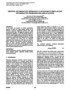
X = random variable denoting the demand during the lead time, g = the probability density function of the lead-time demand with mean µL(Q) and standard deviation σ L (Q ) . It is the L(Q)-fold convolution of the daily demand distribution, f(µ, σ). The constraint in (2) guarantees the non-negativity of the safety stock. For fixed lot size, Q, it can be easily shown that TC(Q,r) is convex in the reorder point, r. However, even for normal daily demand distribution, the convexity of the cost function in Q for fixed r cannot be established analytically. In an unpublished work, Hariga showed numerically through many examples that the function TC(Q, r*(Q)), where r*(Q) is the optimal reorder point for given Q, has a well behaved form that is convex. Figure 1 displays this function when the daily demand is normally distributed. 90000
TC(Q, r*(Q))
80000 70000 60000 50000 40000 30000 20000
147
139
131
123
115
107
99
91
83
75
67
59
51
43
35
27
19
11
10000 0
Lot size, Q Figure 1. Variation of TC(Q, r*(Q)) as function of Q
Given that it is extremely difficult to solve analytically the constrained optimization problem in (2), we propose herein a simulation optimization procedure that can be used for any daily demand distribution. When the (Q, r) inventory system is simulated for a period of n days, the total cost can be written as TC (Q , r ) = S N + h n I + π n B ,
where, N : I
total number of orders placed during the period [0, n], :
B :
time-weighted average value of the on-hand inventory, and time-weighted average value of the backordered demand.
Then, the total annual cost is simply computed as ATC =
TC × number of days per year . n
2.1. Simulation Model In this subsection, a description of the AweSim model is given. For a complete description of the AweSim language, interested reader can refer to Pritsker and O‘Reilly [14]. A self-explanatory AweSim network model for the (Q, r) system with lot size dependent lead time is shown in Figure 2 using the data of the illustrative example. The demand is modeled by the CREATE node CRE1, where inter-arrival times corresponds to time between demands (set equal to one day in the simulation model). When a demand arrives in the model at ASSIGN node ASSIGN_1, the variable XX[7], representing daily demand, is assigned a value according to the probability distribution function of the demand with mean µ and a standard deviation σ. Also, in the ASSIGN node ASN1_2, the variable POS, representing
October 2007
The Arabian Journal for Science and Engineering, Volume 32, Number 2B
331
Ibrahim Al-Harkan and Moncer Hariga
the inventory position, is reduced by XX[7]. Then, two branches are taken from node ASN1_2. The first branch goes to GOON node GOON1. Then, one of the two branches is followed depending on the value of the inventory position after being decreased by XX[7] at node ASSIGN_1 for each demand occurrence. If POS is greater than the reorder point r, no further action is required. However, if POS is reduced to r or lower, then, the reorder process is initiated. An order is placed by first increasing the inventory position, POS, by the number of units ordered, Q, at node ASN2. In addition, at node ASN2, the variable L, representing the lead-time duration, is assigned a value computed from Equation (1). Then, activity number 5, whose duration represents the lead-time before the order arrives, can start. After a period of length L, the order arrives at a GOON node, just after activity 5, where one of the two branches is taken depending on the backorder level. The backorder level is checked to determine the quantity needed to clear backorders, with the remaining units of the lot size becoming part of the inventory. The conditional branching emanating from the GOON node places all the Q units ordered into stock at node ASN5 in case of zero backorders. On the other hand, if BACKO, representing outstanding backorders, is positive, then it is reduced by Q units at node ASN6. If BACKO remains positive or zero after this reduction, then, the ordering lot size is not enough to clear all backorders. Consequently, no change is made to STOCK and no action is taken until the next order arrives. However, if BACKO is negative, then, all backorders are cleared. In this case, the absolute value of BACKO is assigned to STOCK and the variable BACKO is reset to zero at ASSING node ASN7.
Figure 2. AweSim network model for the inventory problem
332
The Arabian Journal for Science and Engineering, Volume 32, Number 2B
October 2007
Ibrahim Al-Harkan and Moncer Hariga
The second branch that emanates from node ASN1_2, goes to GOON node GOON2. Then, one of the two branches is taken according to the variable STOCK, representing the level of stock on hand. If STOCK is greater than or equal to XX[7], then, some units are left in stock and XX[7] units are passed to customers. This action is accomplished at ASSIGN node ASN3 where STOCK is reduced by XX[7]. If STOCK is less than XX[7], then, the excess demanded units are added to the backorder level at ASSIGN node ASN4 and STOCK is reset to zero. The Visual SLAM control statements are exhibited in Appendix 1. The model employs seventeen XX variables as defined in LIMITS statement (line 2). Moreover, the EQUIVALENCE statement allows the use of generic names for the variables instead of AweSim variable names, functions, and constants (lines 4 to 8). In addition, the initial values for the variables are entered using the INTLC statement (lines 12 to 15). The TIMST statement is used to collect timeaveraged statistics on the on hand inventory, backorders, and total number of orders (lines 9, 10, and 11). The inventory system is simulated for a period of ten years (2500 days) to obtain statistics on the above mentioned variables as stated in the INITIALIZE statement (line 17). In order to reduce the bias in the statistics due to the initial starting conditions, replication/deletion approach for means is used (for a complete description of the approach see Law and Kelton [15]). The GENERAL statement is used to input the number of times every scenario (i.e., for specific Q and r) of the inventory system is replicated. In addition, all statistics are to be deleted (cleared) at the end of the first year of the ten-year simulation period. The MONTR statement with CLEAR option (line 18) performs the clearing of statistics. This statement causes all statistical arrays to be cleared after 250 days. Therefore, a warm-up period of 250 days was used to mitigate the effect of initialization bias and, consequently, the statistical results from the simulation model are based on values recorded during the last 2250 days of the simulation run. At the end of every k runs, where k is the number of replications, a call is made automatically to the subroutine OTPUT. Referring to Figure 2, a call is made to subroutine OTPUT by the GOON node labeled OTPUT. Then, whenever this call is made, the total cost is computed in the ASSIGN node labeled COST_EQU,. Next, a series of COLCT nodes is employed where statistics over the k runs are collected on the total cost, the average on hand inventory, the average backorder, and the total number of orders. Note that during the search procedure, 30 replications of the simulation model are made for each scenario of (Q, r). At the end of the simulation optimization procedure, the final least cost solution is run in the simulation model for 50 replications to get a better estimate of the total cost. After building the simulation model, we performed step-by-step debugging to ensure that it is running as intended. We also made several pilot runs to collect simulation statistics and to verify that the simulation model is generating accurate measures of the inventory system performances. 2.2. Simulation Optimization Procedure In this subsection, we outline the simulation optimization procedure, which integrates the AweSim model with a search procedure to find the least-cost ordering quantity and reorder point. Several non-gradient techniques have been proposed to interface with simulation routines to search for the optimal decision variables of complex problems. The Hooke and Jeeves method and the Nelder–Mead method are the most cited techniques in the literature (Haddock and Bengu [10] Swisher et al. [11], Humphry and Wilson [16]). However, these methods require a judicious choice of the starting point and other method specific parameters such as the step size, reflection, expansion, and contractions coefficients. The search procedure we present here is a partial enumeration method that exploits the convexity feature of the cost function in the variables Q and r in an attempt to reduce the number of alternatives to compare. It should be mentioned here that our search procedure generates an approximate solution since the convexity property of the cost function cannot be established for any type of demand distributions. The algorithm searches for the least-cost ordering quantity over the interval [aQ0, bQ0], where Q0 is the economic ordering quantity. Note that we used a search interval for Q containing the economic order quantity (EOQ) value, Qo, since it was established in the literature that the use of the EOQ as the order quantity in the classical (Q, r) model does not lead to substantial deviation from the optimal cost (Zheng [17]). In the first step of the algorithm, the parameters a, b, and mQ can be selected to make the search very exhaustive (small a and large mQ and b). However, this type of selection will be at the expense of the computational effort. In the second step of the algorithm, the search for r is made over the values that are larger than the expected lead-time demand to satisfy the constraint in (2). In the same step, a call is made to the simulation model for each combination of Q and r. The last two steps are improvement steps after finding an initial best solution in Step 2.
October 2007
The Arabian Journal for Science and Engineering, Volume 32, Number 2B
333
Ibrahim Al-Harkan and Moncer Hariga
The steps of the search procedure are outlined next in an algorithmic form. Step 0:
Set Qo =
2S µ , h
TC = M, M is a very large number. Qmin = a Qo, with 0 < a < 1 Step 1:
Qmax = b Qo, with b > 1
∆Q = (Qmax - Qmin)/mQ, where mQ is the number of Q values to be tested. Step 2:
For Q = Qmin to Qmax step ∆Q L(Q) = (PQ + θ) δ rmin = µ L(Q), rmax = 2 rmin, ∆r = rmin/mr , where mr is the number of r values to be tested. TC (Q) = M For r = rmin to rmax step ∆r Call the AweSim model with initial inventory position equal to Q+r and compute TC(Q, r) as the average total cost from 30 replications of the simulation model. If TC(Q, r) < TC (Q) Set TC(Q) = TC (Q, r), Qo = Q, and ro = r Else: exit the r Loop Next r If TC(Q) < TC, set TC = TC(Q), Q* = Qo, and r* = ro Else: exit the Q Loop Next Q Set Qmin = Q*-∆Q , Qmax = Q* + ∆Q, mQ ← mQ/2,
Step 3:
and ∆Q← 2∆Q/mQ Repeat steps 2.
Step 4: Run the simulation model for 50 replications using (Q*, r*) to get a better estimate of TC(Q*, r*) 3. ILLUSTRATIVE EXAMPLES In order to illustrate the combined simulation-optimization procedure described in the previous section, we solve three problems with different daily demand distributions. We first use the normal distribution to validate our model since the approximate (Q, r) problem is analytically solvable for this distribution (see Kim and Benton [5] and Hariga [6]). In the second example problem, we use a Gamma daily distribution for which an analytical solution is extremely difficult. Finally, the case for which an analytical solution is not available is illustrated with a Lognormal distribution. In the three examples, we used a = 0.2, b = 2, mQ = mr = 20. 3.1. Normal Daily Distribution For the purpose of comparison, we use the same example of Kim and Benton [5] and Hariga [6]. The data for this example are as follows: µ = 20 units per day, h = $0.5 per unit per day, π = $600 per unit short, θ = 0.125 day, S = $125, P = 0.025 day per unit, and δ = 10.
334
The Arabian Journal for Science and Engineering, Volume 32, Number 2B
October 2007
Ibrahim Al-Harkan and Moncer Hariga
We report in Table 1 the results of the comparison between our output and that of the analytical approximate model of Hariga [6]. The comparison shows that the simulation optimization model provides accurate measures for the cost performance of the inventory system. In fact, the simulation results exhibits little deviation from the analytical results for the different values of the standard deviation (maximum absolute cost deviation of 2.99%). Moreover, except for the case when σ =5, the integrated simulation-optimization model generated larger values for the ordering quantity, reorder point, and safety stock than the analytical model for all the remaining values of the standard deviation. Table 1. Results of the Comparison Between the Analytical and Simulation Solutions σ
5 8 10 15 22
Solution
Q
Safety
r
Stock
Annual
Annual
Annual
Ordering
Holding
Shortage
Cost
Cost
Cost
ATC
Analytical
77.75
475.67
61.91
8038.51
12599.20
863.48
21501.20
Simulation
58
365
50
10782.22
9863.84
867.16
21513.22
Analytical
68.53
462.48
94.81
9119.43
16134.19
1288.83
26542.46
Simulation
70
471
96
8964.44
16210.79
592.22
25767.45
Analytical
63.56
9833.48
18402.78
1545.48
29781.74
Simulation
70
495
120
9170
18149.52
1690.01
29009.53
Analytical
53.96
458.43
163.62
11582.11
23824.81
2120.88
37527.80
Simulation
58
515
200
12251.67
23243.56
909.52
36404.75
Analytical
44.89
474.70
225.26
13923.26
30962.98
2818.76
47704.99
Simulation
56
605
300
15201.94
27138.78
6165.83
48506.56
458.24 115.44
3.2. Gamma Daily Distribution Suppose that the daily demand, x, follows a Gamma probability density function, p.d.f., with a shape parameter α and scale parameter β. Then, the lead-time demand is also Gamma distributed but with different parameters, as stated in the following property. Property. If the daily demand follows a Gamma (α, β) p.d.f., then the demand over a lead-time of length L(Q) follows also a Gamma (αL(Q), β) with p.d.f α L (Q ) −1
⎛x ⎞ g (x ) = ⎜ ⎟ ⎝β ⎠
e
−
x
β
(3)
βΓ (α L (Q ) )
where Γ[.] is the Gamma function. It is clear that the optimal (Q, r) solution after substituting (3) into (2) is extremely difficult to obtain analytically by minimizing TC(Q, r). Therefore, our simulation optimization procedure is a better alternative to generate a least-cost ordering policy without approximating any of the cost components. To implement our simulation model using a Gamma distribution, we used the same data of the above example problem. The parameter of the Gamma distribution are α = 16 and β = 1.25 which give the same values for the mean and standard deviation (µ = 20 and σ = 5). The results for the Gamma daily demand are summarized in Table 2. Table 2. Results for the Gamma Distribution
October 2007
Q
r
Annual ordering cost
Annual holding cost
Annual shortage cost
Annual total cost
70
435
8939.44
11837.13
800.36
21576.93
The Arabian Journal for Science and Engineering, Volume 32, Number 2B
335
Ibrahim Al-Harkan and Moncer Hariga
3.3. Lognormal daily demand When the daily demand follows a Lognormal distribution, an analytical solution is not available since no specific form for the demand distribution over a lead-time of length L(Q) can be obtained analytically. Again, for such a situation, our simulation optimization procedure can be used to generate a least-cost ordering quantity and reorder point. Using the same data as in the previous two illustrative examples with the parameters of the Lognormal given as α(mean of log x) = 2.876 and β(standard deviation of log x) = 0.2462. These parameter values are selected so that they give the same values for the mean and standard deviation (µ = 20 and σ = 5). The results for this illustrative example are shown in Table 3. Table 3. Results for the Lognormal Distribution Q
r
Annual ordering cost
Annual holding cost
Annual shortage cost
Annual total cost
70
435
8928.06
11901.52
869.07
21698.64
3.4. Experimental study To study the effects of the variability of daily demand and the types of probability density function used on the cost performance of the inventory system, we conducted an experimental study. This experimental work consists of running our simulation optimization procedure using different values of the coefficient of variation (Cv = standard deviation / mean = 0.25, 0.4, 0.5, 0.75, 1.1) for each of the three p.d.f. used in the illustrative example. The results of this work are reported in Table 4. Table 4. Results of the Experimental Study cv=σ/µ
0.25
0.4
0.5
0.75
1.1
Distribution Normal Log Normal Gamma Normal Log Normal Gamma Normal Log Normal Gamma Normal Log Normal Gamma Normal Log Normal Gamma
Q
r
Safety Stock
58 70 70 70 64 58 70 32 58 58 44 38 56 56 44
365 435 435 471 441 415 495 293 435 515 421 362 605 565 397
50 60 60 96 96 100 120 108 120 200 176 147 300 260 152
Annual Holding Cost 9863.84 11901.52 11837.13 16210.79 16054.54 16090.68 18149.52 15333.33 18573.51 23243.56 24587.71 20713.80 27138.78 35750.63 21155.14
Annual Shortage Cost 867.16 869.07 800.36 592.22 2781.99 791.56 1690.01 3386.45 3048.28 909.52 12897.52 6928.99 6165.83 84516.60 214303.59
Annual Average Ordering Total Cost Cost 10782.22 21513.22 8928.06 21698.64 8939.44 21576.93 8964.44 25767.45 9757.22 28593.75 10790.56 27672.79 9170.00 29009.53 19518.06 38237.84 10792.22 32414.01 12251.67 36404.75 14191.67 51676.90 16301.67 43944.46 15201.94 48506.56 11145.56 131412.79 14274.17 249732.90
From Table 4, we can observe that the form of the daily demand distribution does not affect much the system cost performance as well as the ordering policy (Q, r) for small coefficient of variations (cv ≤ 0.4) . However, the choice of the daily demand distribution has a great effect on the ordering policy, and consequently on the cost performance, for cv ≥ 0.5. From the same table, we can also notice that shortage cost component is the most affected by the selection of the demand distribution. For the standard inventory (Q, r) model, Lau and Zaki [18] also found that the shape the lead-time demand distribution significantly affects the shortage cost component of the cost function. Based on the above result of our experimental study, we can conclude that the optimal ordering policy depends on the coefficient of variation and the shape of the daily demand distribution for the continuous review system with lead-time and lot size interaction.
336
The Arabian Journal for Science and Engineering, Volume 32, Number 2B
October 2007
Ibrahim Al-Harkan and Moncer Hariga
4.
CONCLUSIONS
In this paper, we developed an integrated simulation optimization model for the continuous review (Q, r) inventory system with lead-time depending on lot size. We used a linear functional relationship to compute the lead-time for a given lot size. We also illustrated the developed model with three types of demand distributions. Our simulation optimization procedure can be used as a sensitivity analysis tool to study the effects of changes in some problem inputs parameters such as the coefficients of the different cost components and demand distributions. In an underway research work, we are studying the continuous review (Q, r) inventory problem with a stochastic relationship between lead-time and lot size. We assume that the lead-time can be written as the sum of the productive time (run time + setup time) and a random variable representing non-productive time such as moving and waiting times. ACKNOWLEDGEMENTS The authors would like to thank the graduate student Khalid Al-Sitt for his valuable assistance in conducting most of the computational work. The authors would like also to extend their thanks to the two anonymous referees for their valuable comments and suggestions which improved the contents and the presentation of the paper. REFERENCES [1]
R. J. Schonberger, Japanese Manufacturing Techniques: Nine Hidden Lessons in Simplicity. New York: The Free Press, 1982.
[2]
E. Silver, “Changing The Givens in Modeling Inventory Problems: The Example of Just-In-Time Systems”, International Journal of Production Economics, 26(1992), pp. 347–351.
[3]
E. Silver, “Modeling In Support of Continuous Improvement Towards Achieving World Class Operations”, Perspectives in Operations Management, Massachusetts: Kluwer Academic Publishers, 1993, pp. 23–44.
[4]
E. Silver, D. F. Pyke, and R. Peterson, Inventory Management and Production Planning and Scheduling, New York: John Wiley & Sons, 1998.
[5]
J. S. Kim and W. C. Benton, “Lot Size Dependent Lead Times in a Q, R Inventory System”, International Journal of Production Research, 33(1995), pp. 41–58.
[6]
M. Hariga, “A Stochastic Inventory Model with Lead Time and Lot Size Interaction”, Journal of Production Planning and Control, 10(1999), pp. 434–438.
[7]
J. Browne, “Analyzing the Dynamics of Supply and Demand for Goods and Services”, Industrial Engineering, 1994 (June), pp. 18–19.
[8]
J. Banks and C. O. Malave, “The Simulation of Inventory Systems: An Overview”, Simulation, 1984 (June), pp. 283– 290.
[9]
Banks J. and J. P. Spoerer, “Inventory Policy for Continuous Review Case: A Simulation Approach”, The Annals of the Society of Logistics Engineers, 1 (1986), pp. 51–61.
[10]
J. Haddock and G. Bengu, “Application of a Simulation Optimization System for a Continuous Review Inventory Model”, Proceeding of the 1987 Winter Simulation Conference, pp. 382–390.
[11]
J. Swisher, P. D. Hyden, S. H. Jacobson, and L. W. Schruben, “A Survey of Simulation Optimization Techniques and Procedures”, Proceedings of the 2000 Winter Simulation Conference, pp. 119–128.
[12]
Y. Carson and A. Maria, Simulation Optimization: Methods and Applications, Proceeding of the 1997 Winter Simulation Conference, pp. 118–126.
[13]
G. Hadley and T. M. Whitin, Analysis of Inventory Systems. New Jersey: Prentice Hall, Inc., 1966.
[14]
A. Pritsker and J. O'Reilly, Simulation with Visual SLAM and AweSim. 2nd edn. New York: John Wiley & Sons, 1999.
[15]
A. Law and D. Kelton, Simulation Modeling and Analysis, 3nd edn. New York: McGraw-Hill Inc., 2000.
[16]
D. G. Humphrey and J. R. Wilson, “A Revised Simplex Search Procedure for Stochastic Simulation Response Surface optimization”, INFORMS Journal on Computing, 12(4)(2000), pp. 272–283.
[17]
Y. S. Zheng, “On Properties of Stochastic Inventory Systems”, Management Science, 38(1992), pp. 87–103.
[18]
H. S. Lau and A. Zaki, “The Sensitivity of Inventory Decisions to the Shape of the Lead-Time Demand Distribution”, IIE Transactions, 14(1982), pp. 265–271.
October 2007
The Arabian Journal for Science and Engineering, Volume 32, Number 2B
337
Ibrahim Al-Harkan and Moncer Hariga
APPENDIX Control Statements of the Inventory Problem 1
GEN,"(Q, r) Problem ",15/4/2003,100000,YES,YES;
2
LIMITS,26,2;
3
REPORT,80,YES,YES,NONE;
4
EQUIVALENCE,{{POS,XX[1]},{r,XX[2]},{Q,XX[3]},{STOCK,XX[4]}, {BACKO,XX[5]},{TBD,1}};
5
EQUIVALENCE,{{TotalOrder,xx[24]},{AvgBackOrder,xx[23]}, {AvgInvOnHand,xx[22]}};
6
EQUIVALENCE,{{L,XX[6]},{P,XX[9]},{Theta,XX[10]},{Zeta,XX[11]},{pi,xx[25]}};
7
EQUIVALENCE,{{mu,XX[20]},{mR,XX[26]},{mQ,XX[19]},{a,XX[18]}, {h,XX[15]}};
8
EQUIVALENCE,{{b,XX[16]},{s,XX[17]},{TotalCost,XX[13]}};
9
TIMST,1,STOCK,"AvgInvOnHand",0,0.0,1.0;
10 TIMST,2,BACKO,"AvgBackOrder",0,0.0,1.0; 11 TIMST,3,NNCNT(4),"TotalOrder",0,0.0,1.0; 12 INTLC,{{mu,20},{mQ,15},{mR,30}}; 13 INTLC,{{POS,R+Q},{STOCK,R+Q},{BACKO,0}}; 14 INTLC,{{P,0.025},{Theta,0.125},{Zeta,10}}; 15 INTLC,{{h,0.5},{b,2},{s,125},{a,0.2},{pi,600}}; 16 NET; 17 INITIALIZE,0.0,2500,YES,5,NO; 18 MONTR,CLEAR,250; 19 FIN;
338
The Arabian Journal for Science and Engineering, Volume 32, Number 2B
October 2007