371-2008: Count Data Models in SAS - CiteSeerX

SAS Global Forum 2008

Statistics and Data Analysis

Paper 371-2008

Count Data Models in SAS® WenSui Liu, ChoicePoint Precision Marketing, Alpharetta, GA Jimmy Cela, ChoicePoint Precision Marketing, Alpharetta, GA ABSTRACT Poisson regression has been widely used to model count data. However, it is often criticized for its restrictive assumption of equi-dispersion, meaning equality between the variance and the mean. In real-life applications, count data often exhibits over-dispersion and excess zeroes. While Negative binomial regression is able to model count data with over-dispersion, both Hurdle (Mullahy, 1986) and Zero-inflated (Lambert, 1992) regressions address the issue of excess zeroes in their own rights. Different modeling strategies for count data and various statistical tests for model evaluation are illustrated through an example of healthcare utilization. The purpose of this paper is to provide by far the most complete survey of count data modeling strategy in SAS for the user group.

KEYWORDS Poisson regression, Negative binomial regression, Hurdle regression, Zero-Inflated regression, Overdispersion, Excess Zeroes, Vuong test.

1. INTRODUCTION How to model count data as the dependent variable in a regression has become a popular topic in statistics, econometrics, and epidemiology. Deb and Trivedi (1997) modeled the demand for healthcare utilization by the elderly using a finite mixture negative binomial regression. Gurmu (1997) evaluated the impact of managed care program on healthcare utilization using hurdle model. Winkelmann (2004) studied the effect of healthcare reform on the number of doctor visits in Germany using a number of modified count data models. For more detailed discussions about recent development in count data models, please refer to Cameron and Trivedi (2001), Winkelmann and Zimmermann (1995), and Greene (2002). To illustrate models covered in this paper, we use the same data analyzed by Deb and Trivedi (1997). This data is originally obtained from National Medical Expenditure Survey (NMES) conducted in 1987 and includes 4406 respondents who were aged 66 or older and covered by Medicare program. In our example, the number of hospital stays (HOSP) is used as the dependent variable and three types of measures are included in the explanatory variables, which are self-perceived health status (EXCLHLTH, POORHLTH, and NUMCHRON), demographic data (AGE and MALE), and socio-economic information (SCHOOL and PRIVINS). The summary statistics of all variables are given in Table 1. Table 1.1, Variables Used with Summary Statistics Mean

Std. Dev.

HOSP

Variable # of hospital stays

Definition

Obs 4406

0.2960

0.7464

Min 0

Max 8

EXCLHLTH

1 if self-perceived health is excellent

4406

0.0778

0.2680

0

1 1

POORHLTH

1 if self-perceived health is poor

4406

0.1257

0.3316

0

NUMCHRON

# of chronic conditions

4406

1.5420

1.3496

0

8

AGE

age in years (divided by 10)

4406

7.4024

0.6334

6.6

10.9

MALE

1 if the person is male

4406

0.4035

0.4907

0

1

SCHOOL

# of years of education

4406

10.2903

3.7387

0

18

PRIVINS

1 if the person is covered by private insurance

4406

0.7764

0.4167

0

1

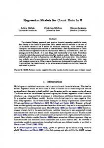
As shown in Table 1.1, the variance of HOSP is about two times of the mean, implying the possibility of overdispersion. A further screening on the data also shows that more than 80% of the respondents, 3541 out of 4406, have no hospital admission, indicating excess zeroes. A good starting point of count data modeling is to compare the empirical distribution of observed counts to the univariate Poisson distribution with the mean estimated from the data. Probabilities from two distributions are plotted in Figure 1.1.

1



Figure 1.1, Comparison between Observed Probability and Univariate Poisson Probability

The plot in Figure 1.1 clearly shows that univariate Poisson distribution underestimates the probability at 0 and overestimates the probability at 1. Since Poisson distribution assumes the same mean across the whole sample and doesn’t consider the heterogeneity in each member, it is not surprising to see that the predicted probability does not fit the observed data well. In the next section, we will allow the observed heterogeneity in the conditional mean of each sample member by including explanatory variables.

2. POISSON REGRESSION Poisson regression is the simplest regression model for count data and assumes that each observed count Yi is drawn from a Poisson distribution with the conditional mean ui on a given vector Xi for case i. Therefore, the density function of Yi can be expressed as

Exp(− ui ) × ui f (Yi | X i ) = Yi !

Yi

, where ui

= Exp( X i β ) .

(2.1)

Given independent observations with the density function in (2.1), the log likelihood function can be obtained by n

LL = ∑ [− ui + Yi Log (ui ) − Log (Yi !)] .

(2.2)

i =1

The maximum likelihood estimation of Poisson regression is straightforward using the log likelihood function in (2.2). In SAS, several procedures in both STAT and ETS modules can be used to estimate Poisson regression. While GENMOD, GLIMMIX, and COUNTREG are easy to use with standard MODEL statement, NLMIXED, MODEL, NLIN provide great flexibility to model count data by specifying the log likelihood function explicitly. An illustration of both NLMIXED and COUNTREG procedures is given below. More detailed examples on how to use all mentioned procedures can be found on author’s blog at statcompute.spaces.live.com. /* METHOD 1: PROC NLMIXED */ proc nlmixed data = tblNMES; parms b0 = 0 b1 = 0 b2 = 0 b3 = 0 b4 = 0 b5 = 0 b6 = 0 b7 = 0; mu = exp(b0 + b1 * EXCLHLTH + b2 * POORHLTH + b3 * NUMCHRON + b4 * AGE + b5 * MALE + b6 * SCHOOL + b7 * PRIVINS); ll = -mu + HOSP * log(mu) - log(fact(HOSP)); model HOSP ~ general(ll); predict mu out = poi_out (rename = (pred = Yhat)); run; /* METHOD 2: PROC COUNTREG */ proc countreg data = tblNMES type = poisson; model HOSP = EXCLHLTH POORHLTH NUMCHRON AGE MALE SCHOOL PRIVINS; run; /* SAMPLE OUTPUT OF PROC COUNTREG: Model Fit Summary Log Likelihood AIC SBC Parameter Estimates 2

-3046 6108 6159



Parameter Intercept exclhlth poorhlth numchron age male school privins

Estimate -3.329044 -0.723412 0.626157 0.264462 0.186406 0.103186 -0.000206 0.108652

Standard Error 0.339728 0.175644 0.067858 0.018277 0.042014 0.056274 0.007871 0.069251

Approx Pr > |t|