3–D Model Construction Using Range and Image Data - Columbia CS

3–D Model Construction Using Range and Image Data

(Submitted to CVPR 2000) ∗

Ioannis Stamos and Peter K. Allen Department of Computer Science, Columbia University, New York, NY 10027 {istamos, allen}@cs.columbia.edu Abstract This paper deals with the automated creation of geometric and photometric correct 3-D models of the world. Those models can be used for virtual reality, tele– presence, digital cinematography and urban planning applications. The combination of range (dense depth estimates) and image sensing (color information) provides data–sets which allow us to create geometrically correct, photorealistic models of high quality. The 3-D models are first built from range data using a volumetric set intersection method previously developed by us. Photometry can be mapped onto these models by registering features from both the 3–D and 2–D data sets. Range data segmentation algorithms have been developed to identify planar regions, determine linear features from planar intersections that can serve as features for registration with 2-D imagery lines, and reduce the overall complexity of the models. Results are shown for building models of large buildings on our campus using real data acquired from multiple sensors.

1

Introduction

The recovery and representation of 3–D geometric and photometric information of the real world is one of the most challenging problems in computer vision research. With this work we would like to address the need for highly realistic geometric models of the world, in particular to create models which represent outdoor urban scenes. Those models may be used in applications such as virtual reality, tele-presence, digital cinematography and urban planning. Our goal is to create an accurate geometric and photometric representation of the scene by means of integrating range and image measurements. The geometry of a scene is captured using range sensing technology whereas the photometry is captured by means of cameras. We have developed a system which, given a set of unregistered depth maps and unregistered photographs, produces a geometric and photometric correct 3–D model representing the scene. We are dealing with all phases of geometrically correct, photorealistic 3–D model construction with a mini∗ This work was supported in part by an ONR/DARPA MURI award ONR N00014-95-1-0601 and NSF grants CDA-96-25374 and EIA-97-29844.

mum of human intervention. This includes data acquisition, segmentation, volumetric modeling, viewpoint registration, feature extraction and matching, and merging of range and image data into complete models. Our final result is not just a set of discrete colored voxels or dense range points but a true geometric CAD model with associated image textures. The entire modeling process can be briefly summarized as follows: 1. Multiple Range scans and 2-D images of the scene are acquired. 2. Each range scan is segmented into planar regions (section 3.1) 3. 3-D linear features from each range scan are automatically found (section 3.2). 4. The segmented range data from each scan is registered with the other scans (section 3.3). 5. Each segmented and registered scan is swept into a solid volume, and each volume is intersected to form a complete, 3-D CAD model of the scene (section 4) 6. Linear features are found in each 2-D image using edge detection methods (section 3.4). 7. The 3-D linear features from step 3 and the 2-D linear features from step 6 are matched and used to create a fully textured, geometrically correct 3-D model of the scene (sections 3.5 and 4). Figure 1 describes the data flow of our approach. We start with multiple, unregistered range scans and photographs of a scene, with range and imagery acquired from different viewpoints. In this paper, the locations of the scans are chosen by the user, but we have also developed an automatic method described in [22] that can plan the appropriate Next Best View. The range data is then segmented into planar regions. The planar segmentation serves a number of purposes. First, it simplifies the acquired data to enable fast and efficient volumetric set operations (union and intersection) for building the 3-D models. Second, it provides a convenient way of identifying prominent 3-D linear features

which can be used for registration with the 2-D images. 3–D linear segments are extracted at the locations where the planar faces intersect, and 2–D edges are extracted from the 2–D imagery. Those linear segments (2–D and 3–D) are the features used for the registration between depth maps and between depth maps and 2–D imagery. Each segmented and registered depth map is then transformed into a partial 3–D solid model of the scene using a volumetric sweep method previously developed by us. The next step is to merge those registered 3–D models into one composite 3–D solid model of the scene. That composite model is then enhanced with 2–D imagery which is registered with the 3–D model by means of 2–D and 3–D feature matching. 2-D Images I1, ..., Im

Range Images R1, ... , Rn

PLANAR SEGMENTATION

Planar Regions P1, ... , Pn 2D LINE EXTRACTION

2-D Line Sets f1, ... fm

MATCH

SOLID SWEEPS

3D LINE EXTRACTION

3-D Line Sets L1, ..., Ln

Partial Solid Models S1, ..., Sn

MATCH

RANGE-IMAGE REGISTRATION

RANGE REGISTRATION

Coordinate Transformations

Position and orientation of images relative to the Final Model TEXTURE MAPPING

INTERSECTION

Final Solid CAD Model

Final Photorealistic Solid Model

Figure 1: System for building geometric and photometric correct solid models.

2

Related work

The extraction of photorealistic models of outdoor environments has received much attention recently including an international workshop [14, 29]. Notable work includes the work of Shum et al. [24], Becker [1, 2], and Debevec et al. [8]. These methods use only 2–D images and require a user to guide the 3-D model creation phase. This leads to lack of scalability wrt the number of processed images of the scene or to the computation of simplified geometric descriptions of the scene which may not be geometrically correct. Teller [6, 18, 26, 5] uses an approach that acquires and processes a large amount of pose–annotated spherical imagery of the scene. This imagery is registered and then stereo methods are used to recreate the geometry. Zisserman’s group in Oxford [11] works towards the fully automatic construction of graphical models of scenes when the input is a sequence of closely spaced 2–D images (video sequence). Both of the previous methods provide depth estimates which

depend on the texture and geometric structure of the scene and which may be quite sparse. Our approach differs in that we use range sensing to provide dense geometric detail which can then be registered and fused with images to provide photometric detail. It is our belief that using 2-D imagery alone (i.e. stereo methods) will only provide sparse and unreliable geometric measures unless some underlying simple geometry is assumed. A related project using both range and imagery is the work of the VIT group [28, 3, 9] The broad scope of this problem requires us to use range image segmentation [4, 13], 3–D edge detection [15, 19], 3–D Model Building [7, 27, 20] and image registration methods [16] as well.

3

System Description

In our previous research, we have developed a method which takes a small number of range images and builds a very accurate 3-D CAD model of an object (see [23, 21] for details). The method is an incremental one that interleaves a sensing operation that acquires and merges information into the model with a planning phase to determine the next sensor position or “view”. The model acquisition system provides facilities for range image acquisition, solid model construction and model merging: both mesh surface and solid representations are used to build a model of the range data from each view, which is then merged with the model built from previous sensing operations. For each range image a solid CAD model is constructed. This model consists of sensed and extruded (along the sensing direction) surfaces. The sensed surface is the boundary between the inside and the outside (towards the sensor) of the sensed object. The extruded surfaces are the boundary between empty sensed 3-D space and un-sensed 3-D space. The merging of registered depth maps is done by means of volumetric boolean set intersection between their corresponding partial solid models We have extended this method to building models of large outdoor structures such as buildings. We are using a Cyrax range scanner which has centimeter level accuracy at distances up to 100 meters to provide dense range sampling of the scene. However, these point data sets can be extremely large (1K x 1K) and computationally unwieldy. The buildings being modeled, although geometrically complex, are comprised of many planar regions, and for reasons of computational and modeling efficiency, these dense point sets can be abstracted into sets of planar regions. In section 4 we present our results of extending this method of automatically building 3-D models to buildings with significant geometry. First we discuss our segmentation methods.

3.1

Planar Segmentation of Range Data

We group the 3–D points from the range scans into clusters of neighboring points which correspond to the

same planar surface. In the Point Classification phase a plane is fit to the points vi which lie on the k × k neighborhood of every point P . The normal np of the computed plane corresponds to the smallest eigenvector T of the 3 by 3 matrix A = ΣN i=1 ((vi − m) · (vi − m)) where m is the centroid of the set of vertices vi . The smallest eigenvalue of the matrix A expresses the deviation of the points vi from the fitted plane, that is it is a measure of the quality of the fit. If the deviation is below a user specified threshold Pthresh the center of the neighborhood is classified as locally planar point. A list of clusters is initialized, one cluster per locally planar point. The next step is to merge the initial list of clusters and to create a minimum number of clusters of maximum size. Each cluster is defined as a set of 3–D points which are connected and which lie on the same algebraic surface (plane in our case). We have to decide if the point P and its nearest neighbors Aj could lie on the same planar surface. If this is the case the clusters where those two points belong are merged into one new cluster. Two adjacent locally planar points are considered to lie on the same planar surface if their corresponding local planar patches have similar orientation and are close in 3D space.

n1 ,

P1

P1

n2 r12

P

,2

P2

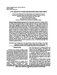
Figure 2: Coplanarity measure. Two planar patches fitted around points P1 and P2 at a distance |r12 | . We introduce a metric of co–normality and co– planarity of two planar patches. Figure 2 displays two local planar patches which have been fit around the points P1 and P2 (Point Classification). The normal of the patches are n1 and n2 respectively. The points Pi0 are the projections of the points Pi on the patches. The two planar patches are considered to be part of the same planar surface if both conditions are met. The first condition is that the patches have identical orientation (within a tolerance region), that is the angle α = cos−1 (n1 · n2 ) is smaller than a threshold αthresh [co–normality measure]. The second condition is that the patches lie on the same infinite plane [co–planarity measure]. The distance between the two patches is defined as d = max(|r12 · n1 |, |r12 · n2 |). This distance should be smaller than a threshold dthresh . r12 is the distance between the projections of P1 and P2 onto their

corresponding local planes. Finally we fit a plane on all points of the final clusters. We also extract the outer boundary of this plane, the convex hull of this boundary and the axis-aligned threedimensional bounding box which encloses this boundary. These are used for fast distance computation between the extracted bounded planar regions whichis described in the next section. Figure 3a is a 2–D image of a building on our campus. Figure 3b shows a point data set from a range scan of this building by a Cyrax scanner from a single view (992 by 989 points). If this data is triangulated into facets, it creates an extremely large, unwieldy, and unnecessarily complex description of an object that is composed of many tiny, contiguous planar surfaces. Our algorithm tries to recover and preserve this structure while effectively reducing the data set size and increasing computational efficiency. Figure 3c shows the segmentation of this data set into planar regions, resulting in a large data reduction - approximately 80% less triangular facets (reduction from 1, 005, 004 to 207, 491 range points) are needed to model this data set. The parameters used were Pthresh = 0.08, αthresh = 0.04 degrees and dthresh = 0.01 meters. The size of the neighborhood used to fit the initial planes was 7 by 7. Points which didn’t pass the first stage of the planar segmentation algorithm and have been classified as non–locally planar are displayed as red.

3.2

3–D Line Detection

The segmentation also provides a method of finding prominent linear features in the range data sets. The intersection of the planar regions provides three dimensional lines which can be used both for registering multiple range images and matching 3-D lines with 2-D lines from imagery. Extraction of 3-D lines is done in three stages: 1. We compute the infinite 3–D lines at the intersection of the extracted planar regions. We do not consider every possible pair of planar regions but only those whose three-dimensional bounding boxes are close wrt each other (distance threshold dbound ). The computation of the distance between two bounding boxes is very fast. However this measure may be inaccurate. Thus we may end up with lines which are the intersection of non-neighboring planes. 2. In order to filter out fictitious lines which are produced by the intersection of non-neighboring planes we disregard all lines whose distance from both producing polygons is larger than a threshold dpoly . The distance of the 3–D line from a convex polygon (both the line and the polygon lie on the same plane) is the minimum distance of this line from every edge of the polygon. In order to compute the

distance between two line segments we use a fast algorithm described in [17]. 3. Finally we need to keep the parts of the infinite 3– D lines which are verified from the data set (that is we extract linear segments out of the infinite 3– D lines). We compute the distance between every point of the clusters Π1 & Π2 and the line L (Π1 & Π2 are the two neighboring planar clusters of points whose intersection produces the infinite line L). We then create a list of the points whose distance from the line L is less than dpoly (see previous paragraph). Those points (points which are close wrt the limit dpoly to the line) are projected on the line. The linear segment which is bounded by those points is the final result. Figure 3d shows 3-D lines recovered using this method and Figure 3e shows these lines overlaid on the 2-D image of the building in Figure 3a after registering the camera’s viewpoint with the range data.

3.3

Registering Range Data

To create a complete description of a scene we need to acquire and register multiple range images. The registration (computation of the rotation matrix R and translation vector T) between the coordinate systems of the nth range image (Cn ) and the first image (C0 ) is done when a matched set of 3–D features of the nth and first image are given. The 3–D features we use are infinite 3–D lines which are extracted using the algorithm described in the previous section. A linear feature f is represented by the pair of vectors (n, p), where n is the direction of the line and p a point on the line. A solution for the rotation and translation is possible when at least two line matches are given. The rotation matrix R can be computed according to the closed form solution described in [10]. The minimization of the error function Σ||ni 0 − Rni ||2 (where ni 0 , ni is the it h pair of matched line orientations between the two coordinate systems) leads to a closed form solution of the rotation (expressed as a quaternion). Given the solution for the rotation we solve for the translation vector T. We establish a correspondence between two arbitraty points on line < n, p >, pj = p + tj n and two points on its matched line < n0 , p0 >, pj 0 = p0 + t0j n0 . Thus we have two vector equations pj 0 = R pj +T which are linear in the three components of the translation vector and the four uknown parameters (tj , t0j ) (2x3 linear equations and 7 uknowns). At least two matched lines provide enough constraints to solve the problem through the solution of a linear overconstrained system of equations. Results of the registration are presented in section 4.

3.4

2–D Line Detection

The computation of 2–D linear image segments is done in the following manner:

1. Application of Canny edge detection with hysteresis thresholding. That provides chains of 2–D edges where each edge is one pixel in size (edge tracking). We used the program xcv of the TargetJr distribution [25] in order to compute the Canny edges. 2. Segmentation of each chain of 2–D edges into linear parts. Each linear part has a minimum length of lmin edges and the maximum least square deviation from the underlying edges is nthresh . The fitting is incremental, that is we try to fit the maximum number of edges to a linear segment while we traverse the edge chain (orthogonal regression).

3.5

Registration of Range and Image Data

We now describe the fusion of the information provided by the range and image sensors. These two sensors provide information of a qualitatively different nature and have distinct projection models. While the range sensor provides the distance between the sensed points and its center of projection, the image sensor captures the light emitted from scene points. The fusion of information between those two sensors requires the knowledge of the internal camera parameters (effective focal length, principal point and distortion parameters) and the relative position and orientation between the centers of projection of the camera and the range sensor. The knowledge of those parameters allows us to invert the image formation process and to project back the color information captured by the camera on the 3–D points provided by the range sensor. Thus we can create a photorealistic representation of the environment. The estimation of the unknown position and orientation of an internally calibrated camera wrt the range sensor is possible if a corresponding set of 3–D and 2–D features is known. Currently, this corresponding set of feature matches is provided by the user but our goal is its automatic computation (see section 5 for a proposed method). We adapted the algorithm proposed by Kumar & Hanson [16] for the registration between range and 2–D images. The input is a set of corresponding 3–D and 2–D line pairs. The internal calibration parameters of the camera are assumed to be known. Let Ni be the normal of the plane formed by the ith image line and the center of projection of the camera (figure 4). This vector is expressed in the coordinate system of the camera. The sum of the squared perpendicular distance of the endpoints e1i and e2i of the corresponding ith 3–D line from that plane is di = (Ni · (R(e1i ) + T))2 + (Ni · (R(e2i ) + T))2 ,

(1)

where the endpoints e1i and e2i are expressed in the coordinate system of the range sensor. The error function we wish to minimize is E1 (R, T) = ΣN i=1 di .

(2)

Figure 3: a) 2-D Image of the scene, b) Range data scan, c) Planar Segmentation (different planes correspond to different colors), d) Extracted 3D lines generated from the intersection of planar regions, e) 3-D lines projected on the image after registration. This function is minimized with respect to the rotation matrix R and the translation vector T. This error function expresses the perpendicular distance of the endpoints of a 3–D line from the plane formed by the perspective projection of the corresponding 2–D line into 3–D space (figure 4). The exact location of the endpoints of the 2–D image segment do not contribute to the error metric and they can move freely along the image line without affecting the error metric. In this case we have a matching between infinite image lines and finite 3–D segments. In the next section we will present results for the complete process of integrating multiple views of both range and imagery.

4

Results

In this section we present results of the complete process: 3–D model acquisition, planar segmentation, volumetric sweeping, volume set intersection, range registration, and range and image registration for a large, geometrically complex and architecturally detailed building on our campus. The bulding is pictured in Figure 5a. Three range scans of the building were acquired at a

Ni

e1i

00 11 1 0 1 0 1 0

e2

11 00 11 00

Image Plane

i

3-D line

Distance of 3-D line’s endpoints from plane formed by corresponding 2-D line and camera’s center of projection.

Camera’s 1 0

2-D line

Coordinate System

Range Sensor’s Coordinate System

R, T

Figure 4: Error metric used for the registration of 3–D and 2–D line sets.

resolution of 976 by 933 3D points. Figures 6a-c show each of these scans, with each data point colored according to the planar region it belongs to from the segmentation process. The parameters used for the segmentation were Pthresh = 0.08, αthresh = 0.04 degrees and dthresh = 0.08 meters. Figure 6d shows the integrated range data set after registering the range images. The range images were registered by manually selecting corresponding 3-D lines generated by the method in section 3.3. Figures 6e-g show the volumetric sweeps of each segmented range scan. These sweeps are generated by extruding each planar face of the segmented range data along the range sensing direction. Volumetric set intersection is then used to intersect the sweeps to create the composite geometric model which encompasses the entire building and is shown in Figure 6h. Figure 6i shows one of the 2-D images of the building (the image shown in Figure5a) texture-mapped on the composite model of Figure 6h. We are calculating the relative position and orientation of the camera wrt to the model as follows: a) the user selects a set of automatically extracted 2–D lines on the 2–D image and its corresponding set of 3–D lines which have also been automatically extracted from the individual depth maps b) the algorithm described in section 3.5 provides the extrinsic parameters of the camera wrt the 3–D model. The internal camera parameters were approximated in this example.

5

of this kind is possible in environments of man–made objects (e.g. buildings) and a result can be seen in figure 5b. More challenging is the automated matching between sets of 3–D and 2–D features. Again the extraction of three directions of parallel 3–D lines (using the automated extracted 3–D line set) and the corresponding directions of 2–D lines (using the automated extracted 2–D line set) can be the first step in that procedure. The knowledge of those directions can be directly used for the solution of the relative orientation between the two sensors. On the other hand extraction of pattern of lines that form windows (which are prominent in the 3–D line set) can lead to the computation of the translation between the two sensors. We have already started incorporating measurements of data uncertainty in our algorithms. Uncertainty in individual range measurements can propagate to the extracted 3–D planes and 3–D lines. Thus, we can have measures of confidence in our extracted features, something that can be used in the automated matching process. As a final step in automating this process, we have also built a mobile robot system which contains both range and image sensors which can be navigated to acquisition sites to create models (described in detail in [12]).

Discussion

We have described a system for building geometrically correct, photorealistic models of large outdoor structures. The system is comprehensive in that includes modules for data acquisition, segmentation, volumetric modeling, feature detection, registration, and fusion of range and image data to create the final models. The final models are true solid CAD models with texture mapping and not just depth maps or sets of colored voxels. This allows these models to be more easily used in many upstream applications, and also allows modeling a wide range of geometry. There are still some areas in which the system can be improved. In some cases our depth maps have gaps due to missed values in transparent parts of the scene (e.g. windows). We handle this by filling the missing data through linear interpolation between the samples that border the gap along a scanline. We would like to extend the system towards the direction of minimal human interaction. At this point the human is involved in two stages: a) the internal calibration of the camera sensor and b) the selection of the matching set of 3–D and 2–D features. We have implemented a camera self–calibration algorithm when three directions of parallel 3–D lines are detected on the 2–D image based on [2]. The automated extraction of lines

Figure 5: a) Image of building, b) Extracted sets of 2–D lines which correspond to parallel 3–D lines. Each set of 2–D lines converges to a distinct vanishing point. The three large axes in the middle of the image point to the corresponding vanishing points.

Acknowledgments We would like to thank Michael K. Reed for help in generating the 3–D models.

References [1] S. Becker and V. M. J. Bove. Semi–automatic 3–D model extraction from uncalibrated 2–D camera views. In SPIE Visual Data Exploration and Analysis II, volume 2410, pages 447–461, February 1995. [2] S. C. Becker. Vision–assisted modeling from model– based video representations. PhD thesis, Massachusetts Institute of Technology, February 1997. [3] J.-A. Beraldin, L. Cournoyer, M. Rioux, F. Blais, S. ElHakim, and G. Godin. Object model creation from multiple range images: Acquisition, calibration, model building and verification. In International Conference on Recent Advances in 3–D Digital Imaging and Modeling, pages 326–333, Ottawa, Canada, May 1997. [4] P. J. Besl and R. C. Jain. Segmentation through variable–order surface fitting. IEEE Transactions on Pattern Analysis and Machine Intelligence, 10(2):167– 192, march 1988. [5] S. Coorg and S. Teller. Extracting textured vertical facades from contolled close-range imagery. In Computer Vision and Pattern Recognition, pages 625–632, Fort Collins, Colorado, 1999. [6] S. R. Coorg. Pose Imagery and Automated Three– Dimensional Modeling of Urban Environments. PhD thesis, MIT, September 1998. [7] B. Curless and M. Levoy. A volumetric method for building complex models from range images. In SIGGRAPH, pages 303–312, 1996. [8] P. E. Debevec, C. J. Taylor, and J. Malik. Modeling and rendering architecure from photographs: A hybrid geometry-based and image-based approach. In SIGGRAPH, 1996. [9] S. F. El-Hakim, P. Boulanger, F. Blais, and J.-A. Beraldin. A system for indoor 3–D mapping and virtual environments. In Videometrics V, July 1997. [10] O. Faugeras. Three–Dimensional Computer Vision. The MIT Press, 1996. [11] A. W. Fitzgibbon and A. Zisserman. Automatic 3D model acquisition and generation of new images from video sequences. In Proceedings of European Signal Processing Conference (EUSIPCO ’98), Rhodes, Greece, pages 1261–1269, 1998. [12] A. Gueorguiev, P. K. Allen, E. Gold, and P. Blair. Design, architecture and control of a mobile site modeling robot. Submitted to IEEE International Conference on Robotics & Automation, April 2000. [13] A. Hoover, G. Jean-Baptise, X. Jiang, et al. An experimental comparison of range image segmentation algorithms. In IEEE Transactions on Pattern Analysis and Machine Intelligence, pages 1–17, july 1996. [14] Institute of Industrial Science(IIS), The University of Tokyo. Urban Multi–Media/3D Mapping workshop, Japan, 1999.

[15] X. Jiang and H. Bunke. Edge detection in range images based on scan line approximation. Computer Vision and Image Understanding, 73(2):183–199, February 1999. [16] R. Kumar and A. R. Hanson. Robust methods for estimating pose and a sensitivity analysis. Computer Vision Graphics and Image Processing, 60(3):313–342, November 1994. [17] V. J. Lumelsky. On fast computation of distance between line segments. Information Processing Letters, 21:55–61, 1985. [18] MIT City Scanning http://graphics.lcs.mit.edu/city/city.html.

Project.

[19] O. Monga, R. Deriche, and J.-M. Rocchisani. 3D edge detection using recursive filtering: Application to scanner images. Computer Vision Graphics and Image Processing, 53(1):76–87, January 1991. [20] R. Pito and R. Bajcsy. A solution to the next best view problem for automated cad model acquisition of free-form objects using range cameras. In SPIE Symposium on Intelligent Systems and Advanced Manufacturing, Philadelphia, October 1995. [21] M. Reed and P. K. Allen. 3-D modeling from range imagery. Image and Vision Computing, 17(1):99–111, February 1999. [22] M. Reed and P. K. Allen. Constraint-based sensor planning for scene modeling. In Computational Intelligence in Robotics and Automation (CIRA99), November 7-9 1999. [23] M. Reed, P. K. Allen, and I. Stamos. Automated model acquisition from range images with view planning. In Computer Vision and Pattern Recognition Conference, pages 72–77, June 16-20 1997. [24] H.-Y. Shum, M. Han, and R. Szeliski. Interactive construction of 3D models from panoramic mosaic. In Computer Vision and Pattern Recognition, Santa Barbara, CA, June 1998. [25] TargetJr standard software http://www.esat.kuleuven.ac.be/˜targetjr/.

platform.

[26] S. Teller, S. Coorg, and N. Master. Acquisition of a large pose-mosaic dataset. In Computer Vision and Pattern Recognition, pages 872–878, Santa Barbara, CA, June 1998. [27] G. Turk and M. Levoy. Zippered polygon meshes from range images. In SIGGRAPH, 1994. [28] Visual Information Technology Group, http://www.vit.iit.nrc.ca/VIT.html.

Canada.

[29] H. Zhao and R. Shibasaki. A system for reconstructing urban 3D objects using ground–based range and CCD sensors. In Urban Multi–Media/3D Mapping workshop, Institute of Industrial Science(IIS), The University of Tokyo, 1999.

Figure 6: Model Building Process: a) First segmented depth map, b) Second segmented depth map, c) Third segmented depth map, d) Registered depth maps, e) First volumetric sweep, f) Second volumetric sweep, g) Third volumetric sweep, h) Composite solid model generated by the intersection of the three sweeps, i) Texture-mapped composite solid model.