Here, we define a piecewise planar scene to be one that comprises a set of ... objects (e.g., building interiors, offices, homes, museums, etc.). This scene prior.
3D Aware Correction and Completion of Depth Maps in Piecewise Planar Scenes Ali K. Thabet1 , Jean Lahoud1 , Daniel Asmar2 , Bernard Ghanem1 1
King Abdullah University of Science and Technology (KAUST), Saudi Arabia 2 American University of Beirut (AUB), Lebanon
Abstract. RGB-D sensors are popular in the computer vision community, especially for problems of scene understanding, semantic scene labeling, and segmentation. However, most of these methods depend on reliable input depth measurements. The reliability of these depth values deteriorates significantly with distance. In practice, unreliable depth measurements are discarded, thus, limiting the performance of methods that use RGB-D data. This paper studies how reliable depth values can be used to correct the unreliable ones, and how to complete (or extend) the available depth data beyond the raw measurements of the sensor (i.e. infer depth at pixels with unknown depth values), given a prior model on the 3D scene. We consider piecewise planar environments in this paper, since many indoor scenes with man-made objects can be modeled as such. We propose a framework that uses the RGB-D sensor’s noise profile to adaptively and robustly fit plane segments (e.g. floor and ceiling) and iteratively complete the depth map, when possible. Depth completion is formulated as a discrete labeling problem (MRF) with hard constraints and solved efficiently using graph cuts. To regularize this problem, we exploit 3D and appearance cues that encourage pixels to take on depth values that will be compatible in 3D to the piecewise planar assumption. Extensive experiments, on a new large-scale and challenging dataset, show that our approach results in more accurate depth maps (with 20% more depth values) than those recorded by the RGB-D sensor. Additional experiments on the NYUv2 dataset show that our method generates more 3D aware depth. These generated depth maps can also be used to improve the performance of a state-of-the-art RGB-D SLAM method.
1
Introduction
Active RGB-D sensors are capable of directly capturing 3D structure from a scene, thus, avoiding the difficult task of inferring this information from the scene’s appearance alone. Sensors like the MS Kinect are popular in computer vision applications, since they are relatively cheap, accessible, and well supported/maintained by manufacturers and third-party developers. There is a large amount of recent work that exploits RGB-D data to generalize and shed light on traditional vision problems, including semantic scene labeling [1], segmentation [2], scene understanding [3–5], object detection [6], visual SLAM (Simultaneous Localization And Mapping) [7, 8], among others.
2
Ali K. Thabet, Jean Lahoud, Daniel Asmar, Bernard Ghanem
Most of the RGB-D methods above rely on the fact that the input depth image is largely comprised of pixels with reliable (accurate) depth measurements. This assumption might not always be valid, as most sensors only provide reliable measurements up to a maximum distance drel (usually of 3-4.5 meters). Given this constraint, most RGB-D based methods either record images where the scene is within the drel range away from the sensor or disregard all pixels whose depth values exceed drel . This unreliability in depth measurement arises due to several reasons, including limitations in the depth sensor itself (e.g., the projected IR signal of a Kinect decays with squared distance and it is unable to image objects that are too close or too far) and the nature of the scene itself (e.g., IR absorbing or reflective surfaces). In Figure 1 (left), we show a sample RGB-D image pair taken in an indoor office scene, with all the unreliable and unknown depth values set to zero (black pixels). Clearly, not all pixels are assigned depth values. Disregarding unreliable pixels limits the range and impedes the generality of methods using RGB-D data. This issue is even more pressing when general indoor scenes are considered, such as in open areas, office spaces, reasonably sized rooms, museums, etc. In these cases, much of the scene is at a distance larger than the maximum reliable depth value drel . We show empirical evidence of this in Figure 1 (right). We histogram the average percentage of pixels discarded in an image because they were deemed unreliable (drel = 4.5 meters) for a typical recording of a walk-through inside an office/lab environment. For this recording, roughly 60% of pixels in each Kinect depth map are deemed unreliable, on average. Discarding such a large number of pixels limits subsequent processing or learning modules, including RGB-D semantic labeling, scene understanding, and visual SLAM methods.
Fig. 1. Left: A sample RGB-D image pair. This is a single frame out of roughly 1000 that were recorded while walking through an indoor piecewise planar scene (office corridor ). Right: The percentage of pixels per image of this walk-through that are unreliable because their depth values are above a certain threshold drel or are unknown.
Interestingly, many of these unreliable pixels are projections of 3D scene points belonging to objects (e.g., floor, ceiling, walls, cabinets, etc.) that have extensions within the reliable range of depth pixels. So, it is important to study how reliable depth values can be used to judge and even correct unreliable ones, when a particular prior model is assumed on the 3D scene. In fact, this could also be used to complete (or extend) the depth values beyond the raw measurements of the sensor itself (i.e., infer depth at pixels with unknown depth). This paper studies this problem for 3D piecewise planar scenes and proposes a novel
3D Aware Correction and Completion of Depth Maps
3
framework that makes use of both appearance and 3D cues from a single RGB-D image pair to correct and complete the depth image. This framework can enable subsequent scene processing and understanding even if the initial RGB-D data is deemed unreliable. Here, we define a piecewise planar scene to be one that comprises a set of intersecting planes (realistically plane segments). Piecewise planar scenes are valid descriptions of many indoor scenes containing man-made objects (e.g., building interiors, offices, homes, museums, etc.). This scene prior has been used in previous work for the purpose of stereo vision or 3D reconstruction [9, 10], semantic labelling [1], and scene understanding from a single RGB-D image [4, 11] or a single RGB image [12–14].
2
Related Work
This paper addresses the problem of correcting unreliable depth values and inferring unknown ones in RGB-D data of piecewise planar scenes. In data of this kind, large groups of contiguous pixels have either unreliable or unknown depth values. The most related work in the literature that address a similar problem (depth enhancement) is categorized as: (1) hole-filling (depth inpainting) methods or (2) depth upsampling methods. Methods of category (1) attempt to infer depth at pixels that are not assigned depth values. These pixels tend to be projections of parts of surfaces that are IR absorbing, reflective, or too close to the RGB-D sensor. These pixels are small in number and tend not to cluster in the same portion of a depth image. Most hole-filling methods interpolate (or propagate) unknown depths from depths in pixel neighborhoods. To this end, joint bilateral filtering (JBF) has been extensively used to fill holes in depth images, especially due to its relatively attractive runtime [15, 16]. Moreover, colorization techniques are also used to fill in unknown depth [17], as done in compiling the popular NYUv2 dataset [18]. In [19], the problem is formulated as a continuous Markov Random Field (MRF), where the latent variables are the depth values of all pixels, the unary (data) term is dependent on the known depth values, and the binary term encourages similar looking pixels in a local neighborhood to have similar depth values. In [20], a foreground depth model is assumed to be available and depth layers are inferred using a discrete MRF. Many other methods of this category exist (e.g., [21]); however, they all suffer from the same drawback that makes them infeasible and inappropriate for the problem of depth correction and completion tackled in this paper. Hole-filling (depth inpainting) methods assume that there is a strong correlation between depth discontinuities and image edges and that pixels with similar appearance have similar 3D geometry. In general, this assumption is a useful cue for interpolation but it does not always hold. It is especially invalid in scenes where large portions of a depth image need to be filled, which is the scope of this paper. Methods of category (2) attempt to generate a high resolution depth image from a low-resolution one and (usually) a registered high resolution RGB image. The low-resolution depth image is usually assumed to be complete and comprising of reliable depth values. Since a plethora of such methods abound
4
Ali K. Thabet, Jean Lahoud, Daniel Asmar, Bernard Ghanem
in the literature, we mention a representative few here. In fact, JBF and MRF labeling are common techniques employed by methods of this category [22, 15, 19]. Similar to the problem of hole-filling, local assumptions of depth smoothness (except at color discontinuities) are made to propagate depth values from the low resolution image to a local neighborhood of unknown values in the higher resolution image. These assumptions break down in the case of large contiguous holes, which makes upsampling methods unsuitable for the problem addressed in this paper. All previous methods apply local priors to depth values in RGB-D data, but they tend not to take into account the global 3D structure of the scene for unreliable depth correction and completion. These methods do not ensure that the processed depth maps lead to a 3D point cloud that has a compatible 3D structure (i.e. its structure does not lead to any 3D contradictions or impossibilities). Assuming a piecewise planar scene allows us to regularize the completion and correction process globally as well as locally. This regularization disallows certain depth assignments that lead to a 3D structure that is not compatible or does not respect the underlying planar assumption. Contributions: They are three fold. (i) Unlike other depth enhancement methods, this paper addresses the problem of correction and completion of unreliable and unknown depth values in a single RGB-D image pair. To the best of our knowledge, this is the first work that makes use of local and global priors on the overall 3D scene to enable 3D aware depth prediction and correction. Here, the global prior on the scene is piecewise planarity. (ii) Instead of discarding unreliable depth information, we make use of its noisy (probabilistic) structure to perform adaptive depth smoothing and adaptive robust plane fitting. We model the depth correction/completion process as a discrete MRF (Markov Random Field), a labeling problem that can be efficiently solved using iterative interactive graph cuts. The unary and binary terms of the MRF go beyond traditional definitions to stress appearance and 3D cues that encourage a 3D structure compatible with the piecewise planar assumption. (iii) To evaluate our proposed approach and validate the importance of depth correction and completion, we compile a challenging, large-scale dataset with ground truth depth. Additionally, we qualitatively evaluate our method on the NYUv2 dataset. Also, we illustrate the merit of our solution in a real-world application, namely RGB-D SLAM. We show that replacing raw depth maps from an RGB-D sensor with our corrected and completed maps substantially improves the performance of a state-of-the-art visual SLAM approach.
3
Proposed Method
In this work, two images generated by an RGB-D sensor (the MS Kinect) are taken as input, where both RGB and depth sensors are assumed to be calibrated (i.e., their intrinsic and extrinsic parameters are estimated beforehand). Denote the RGB and depth images as Ic ∈ RM ×N and Id ∈ RM ×N respectively. In the rest of the paper, we denote Id as the raw depth image, since it contains the unprocessed depth values measured by the sensor directly.
3D Aware Correction and Completion of Depth Maps
3.1
5
Pre-Processing
Before correcting and/or completing depth values in Id , we adaptively smooth them using a precomputed Kinect noise profile (see Supplementary Material) and we robustly extract planar segments from the smoothed 3D data. These segments constitute primitives for the piecewise planar scene, which will subsequently be filtered, grouped, and possibly extended. Adaptive Depth Smoothing: To reduce the effect of sensor noise while preserving depth discontinuities, the projected 3D points are smoothed using the JBF defined in Eq (1). This filter makes use of both the depth image Id and RGB image Ic , as in [20]. Since this filtering method is unaware of the underlying 3D scene, we only use it to smooth existing depth data but not fill unknown depth values in Id . 1 X ˆ Id (q)F (p, q)G(Id (p), Id (q))H(Ic (p), Ic (q)) Id (p) = k
(1)
q∈Ω
In this filter, the smoothed depth at pixel p is a positive weighted sum of the raw depth values in the neighborhood Ω around p. Each weight is a product of three similarity measures between p and its neighbor q: within-image spatial closeness (defined by F ), similarity in raw depth (defined by G), and similarity in appearance (defined by H). Similar to other methods, we take these three functions to be Gaussian. We model G(Id (p), Id (q)) as a Gaussian function N (Id (p) − Id (q), σd (Id (p))), where the standard deviation is depth dependent. By doing this, the JBF is made adaptive to varying depths, which specifically allows for more suitable smoothing at larger depths. Adaptive and Robust Plane Fitting: After depth-adaptive smoothing, we aim to detect and fit 3D planes through the 3D projections of pixels in ˆ Id with known depth. Similar to previous methods, we use RANSAC for robust plane fitting. However, the criterion for a pixel to be an inlier to a fitted plane model (e.g. having the distance of its 3D projection to the plane be less than a threshold) should incorporate the noise in the sensor’s depth measurements. Otherwise, fewer consistent planar segments can be detected at points that are farther away. We start the RANSAC process at pixels with smoothed depth less than drel . We model the actual depth d(p) at pixel p probabilistically as a Gaussian centered around the depth value ˆ Id (p) with a depth-varying standard deviation σd (ˆ Id (p)). Since the depth camera is calibrated, the 3D point corresponding to p is computed as x(p) = d(p)K−1 p ˜ = d(p)t(p), where p ˜ is p in homogenous coordinates and K is the camera matrix. It is easily shown that x(p) is a Gaussian random variable (centered around the observed 3D projection ˆ Id (p)t(p)). Similarly, the distance D(x(p)|(n, n0 )) between x(p) and a 3D plane parameterized by a unit normal n (pointing towards x(p)) and offset n0 also has a Gaussian 2 distribution: D(x(p)|(n, n0 )) ∼ N (µD , σD ), where µD = ˆ Id (p)nT t(p) + n0
2 and σD = σd2 (ˆ Id (p))kn ◦ t(p)k22
(2)
6
Ali K. Thabet, Jean Lahoud, Daniel Asmar, Bernard Ghanem
Note that ◦ is the Hadamard product. As expected, the variance of D(x(p)|(n, n0 )) increases with depth and varies with the relative orientation of the plane with the camera plane. By representing this distance probabilistically, we replace the usual RANSAC inlier condition D(x(p)|(n, n0 )) ≤ a with p(D(x(p)|(n, n0 )) ≤ a) ≥ θ. The latter probability can be computed straightforwardly using the CDF of a Gaussian. In this paper, we take a = 2cm and θ = 0.8. Also, normals of the observed 3D projections ˆ Id (p)t(p) can be used to refine the inliers. Using this probabilistic rule allows a plane model (n, n0 ) that is fit with 3D projections from pixels with reliable depth to extend into farther pixels with less reliable depth. This extension would not be possible and plane fragmentation would ensue, if the conventional RANSAC inlier condition is used. Once the proposed plane-fitting method converges to a set of 3D plane equations and corresponding pixel inliers, we project the 3D projections of the inliers unto their respective planes and update ˆ Id to reflect this projection. This pointto-plane projection changes the depth values acquired by the sensor and, in the majority of cases, corrects their values when a piecewise planar scene is assumed. If a fitted plane exists such that the vast majority of projected points lie in the halfspace designated by its normal and the principal angle between its normal and the normal of the image plane is negative (clockwise), then this fitted plane is designated as the floor. A similar rule determines the ceiling plane, if it exists. 3.2
Depth Completion as an MRF
After pre-processing, the raw depth image Id is transformed into ˆ Id and each pixel with a known depth value is assigned a label corresponding to the fitted plane it belongs to. We denote the resulting label image as L0 ∈ {0, 1, . . . , l}M ×N , where the 0 label designates pixels of unknown depth, 1 the floor (if it exists), and 2 the ceiling (if it exists). In this section, we describe how the initial label image L0 is relabelled through an iterative process that makes use of appearance and 3D cues from Ic and ˆ Id . We denote the label image at iteration k as Lk . As we will see, a consequence of this process is the iterative extension/completion of each plane label and the constriction of the 0 label. In other words, pixels with unknown depth values (labelled 0) can be assigned a plane label, if deemed likely from an appearance and 3D reasoning point of view. We formulate the relabeling process as an iterative interactive graph cuts problem, where regional (unary) and boundary (binary) terms are used to relabel all pixels in the image while enforcing the labels of pixels that already have plane labels. Determining Background Pixels: Clearly, not all pixels in ˆ Id are projections of 3D points that belong to the l fitted planes. Due to sensor limitations and scene structure, other planes might exist in the 3D scene but they are not imaged at all. To allow pixels not to belong to the l fitted planes, we construct a background label, denoted as (l+1). Since no depth information exists for background pixels, we label them according to how their projection rays (3D rays connecting the pixels to the camera’s optical center) relate to the fitted 3D planes, as follows. A pixel is given an (l + 1) label if (i) it cannot belong to any of the l fitted
3D Aware Correction and Completion of Depth Maps
7
planes (i.e. its projection ray does not intersect any of the planes) or (ii) the intersection between its projection ray and each plane j is at least dmax far from the closest known 3D point of plane j. In our experiments, we take dmax = 1 meter. Condition (ii) assumes that the farther away a point is from the observed points on the fitted planes, the more likely it belongs to the background label. Background pixels are labeled as (l + 1) and added to L0 . Figure 2 shows an example of pixels labelled as background in a sample depth frame after plane fitting.
Fig. 2. Left: Original RGB image of a piecewise planar scene. Middle: Initial labeling of plane segments using our robust plane extraction in 3D (background not included). Right: The original RGB image showing only the pixels that are initially labelled in L0 as background.
Discriminative Appearance Model: We discriminatively model the appearance of each label (i.e. pixels whose 3D points belong to the same fitted plane). All labelled pixels in the image are represented using a set of low-level image features that describe a pixel’s color (local color histogram), neighborhood structure (HOG features), and texture information (LBP features). Using PCA, dimensionality reduction is performed to maintain 90% variance in the labelled data. A discriminative appearance model is formed by training a multiclass RBF SVM classifier on all labelled pixels. This model is a vector scoring function h(z) ∈ Rl+1 , where hi (z) is the SVM score of labelling feature vector z as i, for all i ∈ L such that L = {1, . . . , l + 1}. Vanishing Lines: Apart from appearance, other cues exist that shed light on the 3D structure of the scene. A widely used cue is the existence of vanishing line segments. This cue has been extensively used in scene recognition and understanding from single RGB images, especially in indoor piecewise planar scenes [13]. In an image, vanishing points are usually extracted through a process of clustering line segments that vanish to the same point. However, in our case, we can explicitly compute certain vanishing points without any need for clustering or line detection. In indoor scenes, many plane segments tend to be perpendicular to each other (e.g. the floor and walls), thus, many parallel 3D lines in the scene (belonging to the same or different planes) tend to be perpendicular to another plane in the scene. Therefore, we can easily estimate the vanishing point of 3D parallel lines that are perpendicular to fitted plane i by simply constructing at least two such lines (parallel to the normal of plane i) and projecting them unto
8
Ali K. Thabet, Jean Lahoud, Daniel Asmar, Bernard Ghanem
the RGB image Ic . We denote these vanishing points as V1 = {vi }li=1 , where vi is the vanishing point of parallel 3D lines that are perpendicular to plane i. We also use a method similar to [23] to obtain another set of vanishing points V2 that is disjoint from V1 . We maintain a record of the clustered line segments that vanish to points in V1 and V2 . Obviously, the process of extracting line segments and clustering vanishing points in V2 is prone to error, but it provides an additional 3D cue that can be harnessed in the relabeling process. MRF Formulation: Given the label image L0 , we now aim to label all pixels in ˆ Id , especially those with unknown depth values. We model this labelling problem with a discrete Markov Random Field (MRF), where L = {1, . . . , l + 1} is the set of discrete labels, P is the set of all pixels, and E is the set of all connections defining local neighborhoods around each pixel. In our experiments, we consider an 8-connected neighborhood. We seek a labeling f ∗ that minimizes the energy in Eq (3). E(f ) =
X p∈P
U (fp |p) + λ
X
B(p, q)
(3)
(p,q)∈E
Here, U (fp |p) defines the unary (or data) term, which quantifies the cost incurred when pixel p is assigned to label fp ∈ L. Alone, this term treats pixels in ˆ Id independently, so a binary (or smoothness) term B(p, q) is added for regularization, with tradeoff coefficient λ. This term quantifies the cost of assigning neighboring pixels p and q to different labels, i.e. fp 6= fq . This energy can be minimized efficiently using graph cuts [24]. Since some pixels in ˆ Id are already assigned to fitted planes with non-background labels, we use a version of graph cuts (popularly known as interactive graph cuts) to guarantee that the labels of these pixels, after optimization, remain the same. Other optimization methods could be used to solve the normalized version of this problem [25]. Unary (data) Term: Although interactive graph cuts is well-known and has been used for various labelling problems in the past, the quality of the final labeling is mainly determined by how appropriate and informative the unary and binary terms are. Here, the unary term is inversely proportional to the likelihood of a pixel belonging to a fitted plane. This term compares the appearance of a pixel to the discriminative appearance model of each plane and prevents label assignments that are incompatible in 3D under the piecewise planar assumption. In general, we set U (i|p) = −hi (z(p)) for each pixel p ∈ P and each label i ∈ L. This assumes that points belonging to the same plane look similar, which is usually a valid assumption. In what follows, we use 3D cues (from both ˆ Id and ˆ Ic ) to regularize the labelling further. To enforce the hard constraints, we follow a similar strategy as in [24], where U (i|p) = K � 0 for each i ∈ L\{l + 1} and p such that L0 (p) = j 6= i. This large cost K prevents a pixel that is already labelled in L0 to switch labels. This enforcement is done for all labels except background (l + 1), which we allow to constrict or expand. Moreover, we set U (i|p) = K for any pixel p whose projection ray does not intersect plane i. Also, we enforce that all intersections
3D Aware Correction and Completion of Depth Maps
9
between projection rays and planes occur above the floor plane (if it exists) and below the ceiling plane (if it exists). This prohibits label assignments that lead to 3D points, which tunnel into the floor or pierce the ceiling. For these pixels, we set U (1|p) = K and/or U (2|p) = K. Lastly, the unary term should not lead to label assignments that are contradictory in 3D. As such, we set U (i|p) = K for any pixel p, which belongs to a line segment that vanishes to vi ∈ V1 . This discourages p from belonging to a fitted plane, if it lies on a line perpendicular to that plane. In this case, the points belonging to the intersection of two perpendicular planes will be assigned to only one of the two planes and not both. Binary (smoothness) Term: To allow for interactions between neighboring pixels, we define a binary term B(p, q), which encourages label smoothness among pixel neighbors that have similar appearance and/or that are likely to belong to the same plane in 3D. In general, we set B(p, q) = exp(−∆c (p, q)Σ−1 c ∆c (p, q)), where ∆c (p, q) = Ic (p) − Ic (p). The covariance matrix Σc is estimated from Ic . Moreover, we make use of vanishing points to discourage pixels lying on the same vanishing line segment to belong to different planes. So, we set B(p, q) = K when pixels p and q belong to the same line segment that vanishes to a point in V1 P ∪ V2 . In our experiments and as suggested in [24], we set K = 1 + maxp∈P q:(p,q)∈E B(p, q). Iterative Solution: Once all unary and binary terms are computed for all pixels and labels, we solve the labeling problem using interactive graph cuts [24]. Upon convergence, we use the final labeling f ∗ to determine the depth value of each pixel with label fp∗ ∈ {1, . . . , l}. This is done by intersecting the projection ray of p with fitted plane fp∗ . The depth of a pixel labeled as background (i.e. fp∗ = l+1) remains unknown. Effectively, the original label image L0 has been relabelled to produce a modified version L1 . Many pixels that had unknown depth values in L0 have been assigned depth values in L1 . These depth values encourage conformity to appearance models of existing planes and non-contradictory 3D layouts in piecewise planar scenes. In fact, the relabeling process can be rerun with L1 replacing L0 . Obviously, the plane equations can be refined, the appearance model for each label needs to be retrained, and the unary and binary terms should reflect the changes in hard constraints. The resulting iterative relabeling process converges at iteration k when the change in label image δ(Lk , Lk−1 ) is negligible. As such, our proposed approach corrects (through robust plane fitting and projection) and completes (through appearance and 3D aware relabeling) raw depth values recorded by an RGB-D sensor in a piecewise planar scene. In Figure 3, we show how the end-to-end approach applies to a sample pair of RGB-D images.
4
Experimental Results
In this section, we evaluate the effectiveness of our method in enhanceing/correcting and completing depth measurements obtained by the Kinect. For a quantitative comparison between the depth maps generated by our method and the raw depth maps obtained from the sensor, we generate a large-scale 3D point cloud of a
10
Ali K. Thabet, Jean Lahoud, Daniel Asmar, Bernard Ghanem
Fig. 3. End-to-end process. Input: The system takes as input an RGB-D image pair. Pre-processing: The input depth is smoothed using a JBF, after which, plane segments are extracted using the adaptive/robust RANSAC method described in this section. Using the extracted plane segments, an initial label image is created. In addition, background pixels are extracted and added as a new label. In the initial label image, each label is given a distinct color, and orange is used here to describe background pixels. These initial labels are fed to the Graph Cut solver. Output: The final output is a complete set of labels, which are converted to new depth values. We can observe how the depth range is extended from the original 3D point cloud to the final result of our correction/completion process.
typical indoor scene, which we use to generate ground truth depth maps. Additionally, we show some quantitative results on the NYUv2 dataset. We also show how our method can be used in applications like RGB-D slam to enhance its results. 4.1
Dataset Compilation
To create the ground truth set, we scanned a large indoor area using 2 Kinect sensors mounted on a moving platform. The devices were pointed at different fields of view to avoid possible interference of their light patterns. We used 2 devices to be able to cover large areas in the scene, but each device reconstructs its view independently from the other. The relative movement of the platform was constrained to a fixed translation along a predefined direction perpendicular to the floor normal, and a rotation of 0 or ±90◦ around the floor normal; such restrictions make the registration between frames trivial. A total of 700 frames were recorded, corresponding to 220 meters of stretch inside a typical office space. In order to ensure data precision, we select from each frame depth values that only lie within a 0.8 - 4 meters reliable range. The final point cloud size is roughly
3D Aware Correction and Completion of Depth Maps
11
63 million points. Figure 4 shows 2 different views of the final reconstructed point cloud.
Fig. 4. Different views of our large 3D reconstructed dataset. The point cloud covered a physical area of 220 meters and comprised around 63 million points. It contains challenging images of reflective and transparent surfaces, where the Kinect fails to estimate depth values. The depth images obtained are comprised of large gaps with unknown depth as shown in Figure 1.
To create the ground truth frames, we position the point cloud of the whole scene at the local coordinate system of each frame, and we back-project to the image frame using the camera intrinsic parameters; note that the back-projection process creates several 3D candidates for each pixel, but given the scene to camera visibility constraints, the ambiguity is solved by selecting the point closest to the image frame. The depth value at each pixel is the Z coordinate of the projected 3D point. Figure 5 shows a triplet of color, raw depth, and ground truth depth for the same image.
Fig. 5. Left to right: RGB, raw depth, and ground truth depth. We notice the large amount of points missing in the raw depth image, due to the sensor’s inability to process large dark areas and reflective surfaces. The ground truth depth frame shows a complete version of the view by back-projecting the large 3D point cloud aligned to this frame’s view.
4.2 Quantitative Comparison Using the ground truth set, we test the accuracy of our approach and compare it to the raw data provided by the Kinect. The result of our application is a new set of depth frames that improve the raw Kinect data in 2 ways, first by correcting depth values, particularly at large depths, and second by increasing the number of available depth pixels. In order to test for the first hypothesis, we compare the enhanced and raw depth with the ground truth 3D points. The comparison is done by converting the depth values of the enhanced and raw frames into 3D points, and calculating errors as Euclidean distances between closest points of
12
Ali K. Thabet, Jean Lahoud, Daniel Asmar, Bernard Ghanem
these frames and the 3D point cloud of the scene. In order to do this computation in an efficient manner, we build a K-D tree for the ground truth point cloud once, and query the tree using the 3D points of each frame. Figure 6 Left plots these errors for both the raw depth data of the RGB-D sensor and our approach. Our method increases the accuracy of the depth values by an average of 0.5m. We show a wide range of qualitative results on the Supplementary Material.
Fig. 6. Left: Comparison of raw depth values and depth values generated by our method w.r.t. ground truth for a large-scale piecewise planar scene. The plot shows the error per frame in increasing order of error. We notice the significantly lower errors obtained by applying our method. This improvement comes from a combination of correction and completion of the raw depth. Right: Percentage of depth values added to a single image. Our method is adding an average of 50% of depth pixels, and sometimes as much as 80%.
Since our method not only corrects but also extends the depth range of the sensor data; and thus increasing the number of depth pixels available, we also look at the average pixel increase as an additional measure of performance. Figure 6 Right shows a plot of percentage pixel increase per frame, calculated as the percentage of pixels added by the our correction/completion with respect to the original raw data available. The mean increase is around 40000 pixels, with standard deviation of around 20000 pixels. It should be noted at this point that although an increase is present in more than 80% of the cases, the amount of increase always depends on the scene being processed, thus resulting in high standard deviation values. 4.3 Result on NYUv2 Dataset In addition to testing our proposed method on the set we compiled, we also make use of images from the popular NYUv2 dataset [18]. We choose images of piecewise planar environments (such as corridors or hallways) and apply our method on the raw depth images. We compare our corrected and completed depth map to that generated by the hole-filling (colorization) method in [17] used to colorize depth in NYUv2 . We show some examples in Figure 7, where we render 3D views of the raw depth data and the enhanced depth obtained by both techniques. Since the colorization technique is unaware of the 3D structure of the scene, depth points that were added by this method were not constrained to belong to any plane, leading to significant errors. As pointed out in Figure 7,
3D Aware Correction and Completion of Depth Maps
13
these errors come from bad depth predictions at large gaps as well as noise created ad depth discontinuities. Our method does not suffer from these drawbacks due to its 3D aware nature while estimating unknown depth. Further results are available in the Supplementary Material.
Fig. 7. Left to right: 3D renderings of the raw depth, depth after applying the colorization method in [17], depth from our proposed method. The depth colorization method creates unwanted artifacts at large depth gaps (red boxes), as well as a lot of noise at depth discontinuities (green boxes). these problems are not present in our method, since it provides a more 3D aware approach to estimating unknown depth.
4.4
RGB-D SLAM
In order to substantiate the usage of the corrected depth data over regular raw sensor data, we test the performance of a well-known application, the RGBD SLAM, by using the enhanced depth. We tackle the problem of localization in feature-poor environments such as hallways. Such environments are challenging because of the low number of features (SIFTs or SURFs) within the range of the Kinect sensor that could be tracked to estimate the sensor motion. Moreover, using ICP algorithm to estimate the motion in those environments faces convergence to local minima solutions due to the lack of 3D cues. We use a method similar to the one used by [26] with SIFT features. This method can
14
Ali K. Thabet, Jean Lahoud, Daniel Asmar, Bernard Ghanem
be complemented by other methods, such as RGBD ICP by [27], but the goal is to assess the advantages of providing the corrected depth as an input to any application that uses RGBD data. We compare our results to the ground truth data by measuring two errors: the drift in the sensor motion and that of the 3D point locations. The error in 3D point locations is computed as the distance between the predicated 3D point location and the true location where the predicted point location is calculated after movements of 2 meters throughout the hallway. Results are shown in Figure 8. The mean error in point locations is 682mm when using the raw depth and 436mm when using the corrected depth data. For translation, the average drift is 440mm when using raw depth and 283mm when using the our ones. Figure 8 also shows the difference in trajectory between the 2 methods, showing significant improvement when using the corrected/completed depth data.
Fig. 8. RGB-D SLAM comparison. Left: A cumulative density distribution of the frame-to-frame SLAM error when using raw depth and our depth on 700 images. Right: We see in this plot the trajectory estimation of RGB-D SLAM using the raw depth (green), and using our depth (magenta), compared to the original trajectory (black). The improvement (after enhancement) in drift is substantial: 283mm as opposed to 440mm with the raw depth.
5
Conclusion
In this paper we presented a method to use the complete set of depth values provided by an RGB-D sensor to better represent Manhattan environment scenes. We showed that by properly analyzing the sensor error at large depth, we can correct the data given, and segment planar labels from the scene. By applying our method to a new large-scale ground truth data set, we show that our framework provides more accurate depth maps, having a larger number of pixels (20% average increase) than those recorded by the RGB-D sensor. In addition, we qualitatively showed the power of our technique on the NYUv2 dataset. We also applied our methodology to improve the performance of RGB-D SLAM and depth upsampling. Acknowledgement. Research reported in this publication was supported by competitive research funding from King Abdullah University of Science and Technology (KAUST).
3D Aware Correction and Completion of Depth Maps
15
References 1. Koppula, H.S., Anand, A., Joachims, T., Saxena, A.: Semantic Labeling of 3D Point Clouds for Indoor Scenes. In: NIPS. (2011) 244–252 2. Gupta, S., Arbel, P., Malik, J., Berkeley, B.: Perceptual Organization and Recognition of Indoor Scenes from RGB-D Images. CVPR (2013) 3. Barron, J.T., Malik, J., Berkeley, U.C.: Intrinsic Scene Properties from a Single RGB-D Image. CVPR (2013) 4. Jia, Z., Gallagher, A., Saxena, A., Chen, T.: 3D-Based Reasoning with Blocks, Support, and Stability. In: CVPR. (2013) 5. (Gallup, D., Frahm, J.M., Pollefeys, M.) 6. Kim, B.s., Arbor, A., Savarese, S.: Accurate Localization of 3D Objects from RGB-D Data using Segmentation Hypotheses. CVPR (2013) 7. Sturm, J., Engelhard, N., Endres, F., Burgard, W., Cremers, D.: A benchmark for the evaluation of RGB-D SLAM systems. In: IROS. (2012) 573–580 8. Hu, G., Huang, S., Zhao, L.: A robust RGB-D SLAM algorithm. IROS (2012) 1714–1719 9. Furukawa, Y., Curless, B., Seitz, S., Szeliski, R.: Manhattan-world stereo. In: CVPR. (2009) 1422–1429 10. Furukawa, Y., Curless, B., Seitz, S.M., Szeliski, R.: Reconstructing building interiors from images. In: ICCV. (2009) 80–87 11. (Flint, A., Murray, D., Reid, I.) 12. Hedau, V., Hoiem, D., Forsyth, D.: Recovering free space of indoor scenes from a single image. In: CVPR. (2012) 2807–2814 13. Hedau, V., Hoiem, D., Forsyth, D.: Recovering the spatial layout of cluttered rooms. CVPR (2009) 1849–1856 14. Hedau, V., Hoiem, D., Forsyth, D.: Thinking inside the box: Using appearance models and context based on room geometry. (2010) 224–237 15. Kopf, J., Cohen, M.: Joint bilateral upsampling. SIGGRAPH 26 (2007) 16. Camplani, M., Salgado, L.: Efficient spatio-temporal hole filling strategy for kinect depth maps. SPIE (2012) 17. Levin, A., Lischinski, D., Weiss, Y.: Colorization using optimization. In: SIGGRAPH. (2004) 689–694 18. Silberman, N., Hoiem, D., Kohli, P., Fergus, R.: Indoor segmentation and support inference from rgbd images. In: ECCV. (2012) 19. Diebel, J., Thrun, S.: An application of markov random fields to range sensing. NIPS (2005) 20. Cheung, S.c.S.: Layer Depth Denoising and Completion for Structured-Light RGBD Cameras. CVPR (2013) 21. Wang, L., Jin, H., Yang, R., Gong, M.: Stereoscopic inpainting: Joint color and depth completion from stereo images. CVPR (2008) 1–8 22. Park, J., Kim, H., Brown, M.S., Kweon, I.: High quality depth map upsampling for 3D-TOF cameras. (2011) 1623–1630 23. Bazin, J., Seo, Y.: Globally optimal line clustering and vanishing point estimation in manhattan world. In: CVPR. (2012) 638–645 24. Boykov, Y., Funka-Lea, G.: Graph Cuts and Efficient N-D Image Segmentation. IJCV 70 (2006) 109–131 25. Ghanem, B., Ahuja, N.: Dinkelbach NCUT: An efficient framework for solving normalized cuts problems with priors and convex constraints. International Journal of Computer Vision 89 (2010) 40–55
16
Ali K. Thabet, Jean Lahoud, Daniel Asmar, Bernard Ghanem
26. Endres, F., Hess, J., Engelhard, N., Sturm, J., Cremers, D., Burgard, W.: (An evaluation of the RGB-D SLAM system) 27. Henry, P., Krainin, M., Herbst, E., Ren, X., Fox, D.: RGB-D mapping: Using Kinect-style depth cameras for dense 3D modeling of indoor environments. International Journal of Robotics Research 31 (2012) 647–663