At the other two boundaries (x = 110 nun or y = 110 nun) there are thermal exchanges with the environment by convection and radiation. The convective heat ...
lEEE TRANSACTIONSON MAGNETICS, VOL. 27, NO.5, SEPTEMBER 1991 3D FINITE ELEkENT SOLUTION OF INDUCTION HEATING PROBLEMS WITH EFFICIENT Tim-STEPPING
4065
Renato Cardoso Mesquita' & Jolo Pedro Assumpc00 Bastos2
-
I-DEE Universldade Federal de Minas Cerais. AV. do Contorno 842, Centro. 30110. Be10 Horizonte, Mc, BRAZIL
P-CRUCAD/EEVCTC/LFSC. C ~ D U SUniversitario. 88049 Florianbpolis, SC, BRAZIL
-
Abstract A method for the induction heating problem solution in three dimensions is presented. This method couples the transient heat conduction equation associated to convective and radiative boundary condi&ions with the electromagnetic system modeled by the A -$-+ method. The nonlinearities associated to the variation of parameters with the temperature as well as the modeling of the Curie point are also included. Particular attention is given to the time stepping scheme which allows a time-step variation based on the estimation of the error due to time discretization and to the incomplete solution of the problem's nonlinearity. This generates a method which avoids the need of iterative calculations in each time step of the non-linear coupled problem.
Thermal conductivity
Electrical reslstlvity
o
.
o
.
d
,
1
Permeablllty p(T) = a(T1.v 0 x107
l (J/m3/
Introduction
o
'
l
i
l
Curie point
oc)
Thermal ClPaCltY
In the numerical solution of transient induction heating problems, it is generally necessary to solve two systems of equations at each time-step: one electromagnetic and the other thermic. These systems are strongly coupled and non-linear, since the magnetic materials characteristics change with the temperature, and the thermal sources depend on the eddy currents distribution and, normally, the computer's time spent in the solution of the problem is high. In the specific case of three-dimensional induction heating problems, the computer time is even bigger, because there is an increase in the system's dimensions due to the addition of the spatial coordinate and to the vectorial nature of the electromagnetic variables. As such, an efficient method for temporal discretization is a must. In this paper a method for the 3D induction heating problem solution in three dimensions is presented with a time-stepping method which avoids the iterative calculation process of the non-linear coupled problem. Mathematical model
200
,
I
400
,
I
600
t
,
800
,
,
1000
I
,
1200
Temperature (C)
Fig. 1: Physical properties variation regions: in the first, Rj, there are externally imposed currents and the magnetic permeability is uniform and equal to PO; in the second, Ski, there are high permeability magnetic materials, without any kind of currents. The method A*-@-# [31 is used tq model this problem. The modified vector potential A [ 3 1 is used [ 4 1 in in Rr, coupled to the total scalar potential Slk and to the reduced scalar potential # [41 in RJ. The problem is described by the following equations:
*
Thermal modeling - The thermal problem is modeled by the transient heat conduction equation 111, [21: c at + div(-k grad TI
= q
(1)
where c is the thermal capacity, T is the temperature, k is the thermal conductivity and q are the thermal sources. c and k depend on the temperature, as shown in fig. 1. The energy of Curie transition is simulated by a Gaussian exponential variation of c, which is very smooth and gives good results from the physical viewpoint [21. The boundary conditions are convective and radiative, that is: k
an
=
-h(T
-
T 1
-
EI(T'
- T ' )
where Ta is the environment temperature, h is the convective heat transfer. coefficient, E is the emissivity and r is the Stefan-Boltzmann constant. Eddy-currents modeling - Consider the 3D eddy currents problem schematically represented in figure 2. It consists of a conducting region Rf where eddy currents are induced, surrounded by two non-conducting
Fig. 2: Schematic representation of 3-D eddy currents problem The Calerkin method is applied to these equations. To couple the three regions, the continuity of f i n and B.n is enforced at their interfaces [31, [41. The choice of a method to model a 3-D eddy currents problem is not a simple task, and has to be justificated. There are various possibilities for the choice as, for instance, the method A-V-*-# with Coulomb gauge [SI and with Lorentz gauge [SI, the T-R method [71 and the H method [81. In this work we have
0018-9464/91$01.00 0 1991 IEEE
Authorized licensed use limited to: UNIVERSIDADE FEDERAL DE MINAS GERAIS. Downloaded on August 19, 2009 at 11:33 from IEEE Xplore. Restrictions apply.
EEE TRANSACTIONS ON M A C X " ! S ,
4066
selected the A*-$-&
VOL. 27, NO. 5, SEPTEMBER 1991
with the approximations:
based on the following facts:
1. The thermal time constants are many times bigger than the electrical time constants. Then, the electromagnetic calculations can be done as a sequence of sinusoidal electrical steady-states. As the frequency in induction heating problems is equal or even bigger than 50 Hz, the problem sf non-uniqueness associated to low frequencies in the A method [SI does not exist.
(10) (11)
at time te the equation ( 7 ) is approximated by:
In an inductio:i heating problem, q is the power dissipated by the eddy-currents, that is: 2.
q =
1 II
J 11'
(6)
S o , from the thermal point of view, the most important electromagnetic variable is the current density, on whose value we have to obtain the greatest precision.
3 . In the T-R method as well as in the H method, J
is evaluated as: J
= curl T
or
rearranging: [[Cle
+
=
OAt [KTlel
f," -
e 1
[KIl
T.
For the nonlinear case, the met od ha to include $ 0 a prediction step to evaluate T.'*'. 1 , [Cl , . . . , etc, and a subsequent correction step. The algorithm thus obtained is:
J = curl H,
respectively. Then J doesn't have the same prgcision as A method
T or H which are the base variables. In the J = - j w A Then, J has the same precision of A-.
(15) (iii)
re
(iv)
Evaluate [Cle, [KTle, [KEle,
=
(i-e)T'
+
ey'+'
(16)
f,
. . . etc.
4. The pieces to be heated are generally composed by only one kind of material. So it is not necessary for the chosen method to represent discontinuities ig the electrical conductivity (which would exclude the A method). 5. The temperature spatial distribution is continuous. The electrical conductivity and magnetic permeability variations with temperature are also continuous (see fig. 1). Then U and & have continuous spatial changes. Even though the A method doesn't allow the discontinuous variation of U , it permits its continuous variation. 6. Of all the referenced methods, the ones that present the least number .of variables inside the conducting regions are the A and the H.
(18) A nonlinear problem has to be solved iteratively in steps (iii) to (vi) until a convergence in E'+' is obtained. The Newton-Flaphson algorithm can be used to accelerate the convergence process.
Time-step variation - Through the evaluation of the neglected terms in the Taylor series development of a differential equation system with the same structure of (71, Zienkiewicz et al. [lo] obtained an approximated measure of the error at each time-step given as: e
The finite-element model and the time discretization The Galerkin and the finite-element methods can be applied to equations (1) to ( 6 ) to obtain the following semi-discrete form [91: (7)
[KE(T.)I E =
(8)
In these equations, all the terms depend on the temperature vector 1, and LT also depends on the electrical variables vector E. The first order e method [lo] is used for the discretization of the equation ( 7 ) . Consider that in an instant of time ti the values of
1' = T.(t') and E'
= E(t')
are known. The equations ( 7 ) and (8) are written at the time
te =
(13)
t i + BAt
(9)
7
=
(a' - - -a'+')At/2
(19)
The error norm can be used as a criterion for the time-step changes. A reasonable procedure is to reduce (for instance halving) At if the error norm is greater than a certain value, Em, and to increase it (for instance doubling) when the error norm is lower than an fraction of Em. The time-step changing can be used, also, to avoid the non-linear iterative calculations (steps ( i i i ) to (vi) in the algorilthm) at each time-step. The difference between E and a' is only due to the -P
non-linear nature of the problem. Then, the error associated to the incomplete solution of the non-linear problem can be approximately evaluated by 191: (20)
Now, At is reduced if IIg~llor IIe_nll is greater than E m and is increased if IIg~ll and IIgnll are both lower than a fraction of Em. With this new strategy the computer time is strongly reduced. Numerical Example The program was validated through the solution of
Authorized licensed use limited to: UNIVERSIDADE FEDERAL DE MINAS GERAIS. Downloaded on August 19, 2009 at 11:33 from IEEE Xplore. Restrictions apply.
4067
IEEETRANSACTIONS ON MAGNETICS, VOL. 27, NO. 5 , SEPTEMBER 1991 induction heating axisymmetric problems for which there are numerical results obtained from a 2-D program [111. Being certain that the program was performing correctly, the formulation was used in the solution of a modified version of the TEAM Workshops problem 5, the Bath-cube [12]. In this adaptation, the problem geometry is maintained (Fig. 3). as well as the driving freqriency (50 Hz). However, the driving MMF is increased from 1000 A-e to 20000 A-e, and the cube material is changed to the one shown in Fig. 1. With these modifications, the eddy-current intensity and the power density increases and the cube heats up. For the induction heating problem so defined, it is necessary to add thermal boundary conditions, which are specified on the cube surfaces. In this simulation it is supposed that the internal boundaries of the cube (x = 40mm, or y = 40 nun) as well as the top and bottom boundary ( z = 64". o r z = 4 nun) are isolated from the outside world with a thermal isolator. Then, at these boundaries the thermal boundary condition is:
TEMPERATURE ("Cf
POWER DENSITY
t 4500Ef03 40OOEf03 3 .3500E*03 4 .3000E+03 5 .2500E+03 7 .1500E*OI 6 .2OOOE+03
(w/m3)
2
k
8 .lOOOE+03 9 5000E+O2
(a) t = 2.1 s At the other two boundaries (x = 110 nun or y = 110 nun) there are thermal exchanges with the environment by convection and radiation. The convective heat transfer coefficient and emissivity are set, respectively, at h=10 W/(m2 "C) and E = 0.8.
POWER DENSITY (w/m3)
TEMPERATURE ("C)
k
I I
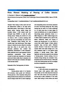
Fig. 3: The Bath-cube geometry. Front view and view from above of the setup (all dimensions in nun). (From Bossavit, [121) Fig 4 shows the temperature and power density distribution on the cube surfaces at t=2.1 s , 13 s and 1877 s . The figure 5 shows the temperature evolution at the points A(x = 70 nun, y = 110 mm, z = 64 nun), B(x = 40 nun, y = 40 mm, z = 64 nun), C(x = 110 mm, y = 110 nun, z = 40 nun) and D(x = 40 mm, y = 70 nun, z = 64 mm) (see also fig. 3). It can be seen that initially (t=2.ls) the entire cube is at low temperature. Then, all of its material is in the magnetic state and the power density is very high on the cube top surface. As the cube goes through the heating process, the power density distribution changes (t=13s): it decreases in points where the temperature approximates the Curie point, because the material becomes nonmagnetic. In these initial instants of time, the points that heat faster are the ones placed on regions with high power density, as the point A, located at the intersection of the top face (z=64nun) and of the external lateral face (y=110 nun) of the cube. As the temperature rises and the power density reduces, this situation changes. The hotest points migrates to the regions far from the faces where there are thermal exchanges with the environment, as the points D and B. The least hot points are situated on the faces where there are thermal exchanges, as the points A and C. It is interesting to note the temperature fall at point A from t=20s to t=200s. That is due to the reduction of the power density in the neighbourhood of
(b)
TEMPERATURE ("C)
t = 13
s
POWER DENSITY (w/m3)
(c) t = 1877 s
Fig. 4 Temperature and power density distribution point A and to thermal exchanges with the environment and with the colder points in the cube. At the steady-state (t-1877s) the point B is the hotest point in the cube and the point C is the coldest. Fig. 6 shows the time-step evolution.
Authorized licensed use limited to: UNIVERSIDADE FEDERAL DE MINAS GERAIS. Downloaded on August 19, 2009 at 11:33 from IEEE Xplore. Restrictions apply.
Authorized licensed use limited to: UNIVERSIDADE FEDERAL DE MINAS GERAIS. Downloaded on August 19, 2009 at 11:33 from IEEE Xplore. Restrictions apply.