Apr 27, 2018 - I also want to thank Joshua Ward for the language revision of the thesis. I am grateful to all my ..... (2009) and Collett et al. (2012) also studied ...
D 1456
OULU 2018
UNIVERSITY OF OUL U P.O. Box 8000 FI-90014 UNIVERSITY OF OULU FINLA ND
U N I V E R S I TAT I S
O U L U E N S I S
ACTA
A C TA
D 1456
ACTA
U N I V E R S I T AT I S O U L U E N S I S
Ville Vuollo
University Lecturer Santeri Palviainen
Postdoctoral research fellow Sanna Taskila
Professor Olli Vuolteenaho
University Lecturer Veli-Matti Ulvinen
Ville Vuollo
University Lecturer Tuomo Glumoff
3D IMAGING AND NONPARAMETRIC FUNCTION ESTIMATION METHODS FOR ANALYSIS OF INFANT CRANIAL SHAPE AND DETECTION OF TWIN ZYGOSITY
Planning Director Pertti Tikkanen
Professor Jari Juga
University Lecturer Anu Soikkeli
Professor Olli Vuolteenaho
Publications Editor Kirsti Nurkkala ISBN 978-952-62-1854-0 (Paperback) ISBN 978-952-62-1855-7 (PDF) ISSN 0355-3221 (Print) ISSN 1796-2234 (Online)
UNIVERSITY OF OULU GRADUATE SCHOOL; UNIVERSITY OF OULU, FACULTY OF MEDICINE; MEDICAL RESEARCH CENTER OULU; OULU UNIVERSITY HOSPITAL
D
MEDICA
ACTA UNIVERSITATIS OULUENSIS
D Medica 1456
VILLE VUOLLO
3D IMAGING AND NONPARAMETRIC FUNCTION ESTIMATION METHODS FOR ANALYSIS OF INFANT CRANIAL SHAPE AND DETECTION OF TWIN ZYGOSITY Academic dissertation to be presented with the assent of the Doctoral Training Committee of Health and Biosciences of the University of Oulu for public defence in the Auditorium of Kastelli Research Centre (Aapistie 1), on 27 April 2018, at 12 noon
U N I VE R S I T Y O F O U L U , O U L U 2 0 1 8
Copyright © 2018 Acta Univ. Oul. D 1456, 2018
Supervised by Professor Pertti Pirttiniemi Docent Tuomo Heikkinen Professor Lasse Holmström
Reviewed by Professor Rosa M. Crujeiras Professor Cheolwoo Park Opponent Professor Fred Godtliebsen
ISBN 978-952-62-1854-0 (Paperback) ISBN 978-952-62-1855-7 (PDF) ISSN 0355-3221 (Printed) ISSN 1796-2234 (Online)
Cover Design Raimo Ahonen
JUVENES PRINT TAMPERE 2018
Vuollo, Ville, 3D imaging and nonparametric function estimation methods for analysis of infant cranial shape and detection of twin zygosity. University of Oulu Graduate School; University of Oulu, Faculty of Medicine; Medical Research Center Oulu; Oulu University Hospital Acta Univ. Oul. D 1456, 2018 University of Oulu, P.O. Box 8000, FI-90014 University of Oulu, Finland
Abstract The use of 3D imaging of craniofacial soft tissue has increased in medical science, and imaging technology has been developed greatly in recent years. 3D models are quite accurate and with imaging devices based on stereophotogrammetry, capturing the data is a quick and easy operation for the subject. However, analyzing 3D models of the face or head can be challenging and there is a growing need for efficient quantitative methods. In this thesis, new mathematical methods and tools for measuring craniofacial structures are developed. The thesis is divided into three parts. In the first part, facial 3D data of Lithuanian twins are used for the determination of zygosity. Statistical pattern recognition methodology is used for classification and the results are compared with DNA testing. In the second part of the thesis, the distribution of surface normal vector directions of a 3D infant head model is used to analyze skull deformation. The level of flatness and asymmetry are quantified by functionals of the kernel density estimate of the normal vector directions. Using 3D models from infants at the age of three months and clinical ratings made by experts, this novel method is compared with some previously suggested approaches. The method is also applied to clinical longitudinal research in which 3D images from three different time points are analyzed to find the course of positional cranial deformation and associated risk factors. The final part of the thesis introduces a novel statistical scale space method, SphereSiZer, for exploring the structures of a probability density function defined on the unit sphere. The tools developed in the second part are used for the implementation of SphereSiZer. In SphereSiZer, the scale-dependent features of the density are visualized by projecting the statistically significant gradients onto a planar contour plot of the density function. The method is tested by analyzing samples of surface unit normal vector data of an infant head as well as data from generated simulated spherical densities. The results and examples of the study show that the proposed novel methods perform well. The methods can be extended and developed in further studies. Cranial and facial 3D models will offer many opportunities for the development of new and sophisticated analytical methods in the future.
Keywords: 3D surface imaging, cranial deformations, directional statistics, head shape, kernel density estimation, scale space, spherical data, statistical pattern recognition, stereophotogrammetry, twin study, zygosity
Vuollo, Ville, Imeväisikäisten pään muodon analyysi ja kaksosten tsygositeetin tunnistus 3D-kuvantamisen ja parametrittomien funktion estimointimenetelmien avulla. Oulun yliopiston tutkijakoulu; Oulun yliopisto, Lääketieteellinen tiedekunta; Medical Research Center Oulu; Oulun yliopistollinen sairaala Acta Univ. Oul. D 1456, 2018 Oulun yliopisto, PL 8000, 90014 Oulun yliopisto
Tiivistelmä Pään ja kasvojen pehmytkudoksen 3D-kuvantaminen on yleistynyt lääketieteessä, ja siihen tarvittava teknologia on kehittynyt huomattavasti viime vuosina. 3D-mallit ovat melko tarkkoja, ja kuvaus stereofotogrammetriaan perustuvalla laitteella on nopea ja helppo tilanne kuvattavalle. Kasvojen ja pään 3D-mallien analysointi voi kuitenkin olla haastavaa, ja tarve tehokkaille kvantitatiivisille menetelmille on kasvanut. Tässä väitöskirjassa kehitetään uusia matemaattisia kraniofakiaalisten rakenteiden mittausmenetelmiä ja -työkaluja. Työ on jaettu kolmeen osaan. Ensimmäisessä osassa pyritään määrittämään liettualaisten kaksosten tsygositeetti kasvojen 3D-datan perusteella. Luokituksessa hyödynnetään tilastollista hahmontunnistusta, ja tuloksia verrataan DNA-testituloksiin. Toisessa osassa analysoidaan pään epämuodostumia imeväisikäisten päiden 3D-kuvista laskettujen pintanormaalivektorien suuntiin perustuvan jakauman avulla. Tasaisuuden ja epäsymmetrian määrää mitataan normaalivektorien suuntakulmien ydinestimaatin funktionaalien avulla. Kehitettyä menetelmää verrataan joihinkin aiemmin ehdotettuihin lähestymistapoihin mittaamalla kolmen kuukauden ikäisten imeväisten 3D-malleja ja tarkastelemalla asiantuntijoiden tekemiä kliinisiä pisteytyksiä. Menetelmää sovelletaan myös kliiniseen pitkittäistutkimukseen, jossa tutkitaan pään epämuodostumien ja niihin liittyvien riskitekijöiden kehitystä kolmena eri ajankohtana otettujen 3D-kuvien perusteella. Viimeisessä osassa esitellään uusi tilastollinen skaala-avaruusmenetelmä SphereSiZer, jolla tutkitaan yksikköpallon tiheysfunktion rakenteita. Toisessa osassa kehitettyjä työkaluja sovelletaan SphereSiZerin toteutukseen. SphereSiZer-menetelmässä tiheysfunktion eri skaalojen piirteet visualisoidaan projisoimalla tilastollisesti merkitsevät gradientit tiheysfunktiota kuvaavalle isoviivakartalle. Menetelmää sovelletaan imeväisikäisen pään pintanormaalivektoridataan ja simuloituihin, pallotiheysfunktioihin perustuviin otoksiin. Tulosten ja esimerkkien perusteella väitöskirjassa esitetyt uudet menetelmät toimivat hyvin. Menetelmiä voidaan myös kehittää edelleen ja laajentaa jatkotutkimuksissa. Pään ja kasvojen 3D-mallit tarjoavat paljon mahdollisuuksia uusien ja laadukkaiden analyysityökalujen kehitykseen myöhemmissä tutkimuksissa.
Asiasanat: 3D-kuvantaminen, epämuotoisuus, kaksostutkimus, pallopinnan data, pään muoto, skaala-avaruus, stereofotogrammetria, tilastollinen hahmontunnistus, tsygositeetti, ydinestimointi
To Ellen and Alisa Once we accept our limits, we go beyond them. – Albert Einstein
8
Acknowledgements This work was carried out at the Department of Oral Development and Orthodontics, Research Unit of Oral Health Sciences, University of Oulu, and at the Oral and Maxillofacial Department, Oulu University Hospital, in close collaboration with the Research Unit of Mathematical Sciences, University of Oulu, between 2014 and 2017. First, I would like to express my sincere appreciation to my supervisors Professor Pertti Pirttiniemi, DDS, PhD, Docent Tuomo Heikkinen, DDS, PhD, and Professor Emeritus Lasse Holmström, PhD. Pertti, you have been the driving force behind this dissertation project. Your valuable work in organizing these 3D studies, despite your many other responsibilities, has made my work much easier, and I have been able to properly focus on this thesis. Tuomo, I owe my deepest gratitude to you for trusting in me and inviting me to this project from the very beginning. I appreciate your guidance on clinical and dental research. Lasse, this is my third thesis with you as my supervisor, and it has been a pleasure to work with you all these years. Your guidance and feedback have been invaluable throughout my studies. I also want to thank the pre-examiners of this thesis, Professors Rosa M. Crujeiras, PhD, and Cheolwoo Park, PhD, for contributing their time and expertise. Your constructive criticism and valuable advice have substantially improved the quality of this thesis. I also want to thank Joshua Ward for the language revision of the thesis. I am grateful to all my co-authors. I would especially like to thank my research group members, Henri Aarnivala, MD, PhD, Docent Virpi Harila, DDS, PhD, and Docent Marita Valkama, MD, PhD, for the professional and personal support. Collecting research material with you provided a refreshing change to my regular days at the office. I would also like to thank my collaborators abroad, Professor Antanas Sidlauskas, DDS, PhD, Mantas Sidlauskas, DDS, PhD, and Alexei Zhurov, PhD. I wish to thank my follow-up group members, Professor Esa Läärä and Leena Ruha, PhD, for their time and experience. I also want to express my gratitude to my fellow statisticians Toni Similä, MSc, and Hannu Vähänikkilä, PhD, and my co-author Henri for their peer support during the doctoral training. The working atmosphere at the Research Unit of Oral Health Sciences has been pleasantly friendly, for which I am truly thankful to all my colleagues.
9
Furthermore, I would like to express my gratitude to the University of Oulu Graduate School (UniOGS) and the Finnish Doctoral Programme in Oral Sciences (FINDOS), which have enabled this thesis. I also acknowledge Finnish Dental Society Apollonia and Planmeca for providing financial support. I am deeply grateful to all the twins in Lithuania and all the children and their families in Finland who participated in these studies. This thesis would not have been possible without their contribution. Finally, I would like to thank my friends and family. My friends, although not directly involved in this work, you have been a great asset to me and have provided me with something else to think about when necessary. The same goes for my wife’s family, which I consider my family, too. My warmest gratitude goes to my parents for their love, encouragement and support during this thesis and throughout my whole life. I dedicate this thesis to my daughter and my wife. Alisa, my dear little daughter, you are the joy of my life, and watching you grow and live is without doubt my most important research project in life. And Ellen, my beloved wife, I have no words to express my gratitude for your constant support, understanding and love throughout all these years. You two have been my greatest resource throughout this work, and I am blessed to be a part of our family.
10
Abbreviations 2D
Two-dimensional
3D
Three-dimensional
AS
Asymmetry score
BIC
Bayesian information criterion
CI
Cephalic index
DZ
Dizygotic
ESS
Effective sample size
FS
Flatness score
HAS
2D histogram asymmetry score
HFS
2D histogram flatness score
MZ
Monozygotic
OCLR
Oblique cranial length ratio
PCAI
Posterior cranial asymmetry index
ROT
Rule of thumb
SiZer
Significant zero crossings of derivatives
wAS
Weighted asymmetry score
11
12
List of original publications This thesis is based on the following articles, which are referred to in the text by their Roman numerals (I–IV): I
Vuollo V, Sidlauskas M, Sidlauskas A, Harila V, Salomskiene L, Zhurov A, Holmström L, Pirttiniemi P & Heikkinen T (2015) Comparing Facial 3D Analysis With DNA Testing to Determine Zygosities of Twins. Twin Research and Human Genetics 18(6): 306–313. II Vuollo V, Holmström L, Aarnivala H, Harila V, Heikkinen T, Pirttiniemi P & Valkama AM (2016) Analyzing infant head flatness and asymmetry using kernel density estimation of directional surface data from a craniofacial 3D model. Statistics in Medicine 35(26): 4891–4904. III Aarnivala H, Vuollo V, Harila V, Heikkinen T, Pirttiniemi P, Holmström L & Valkama AM (2016) The course of positional cranial deformation from 3 to 12 months of age and associated risk factors: a follow-up with 3D imaging. European Journal of Pediatrics 175(12): 1893–1903. IV Vuollo V & Holmström L (2018) A scale space approach for exploring structure in spherical data. Computational Statistics and Data Analysis. In press.
Paper I was co-written and its ideas were co-developed by Docent T. Heikkinen, DDS, PhD, Professor L. Holmström, PhD, and the author. Papers II and IV were co-written and their ideas were co-developed by L. Holmström and the author. Paper III was co-written by the author and H. Aarnivala, MD, PhD, who carried the principal responsibility. Statistical analyses and models in Paper III were designed and conducted by both H. Aarnivala and the author. The artificial data used in Papers II and IV were designed by the author. The author recorded and processed the 3D data and was responsible for implementation of the methods and the computations.
13
14
Contents Abstract Tiivistelmä Acknowledgements
9
Abbreviations
11
List of original publications
13
Contents
15
1 Introduction
17
2 Craniofacial 3D surface imaging
19
2.1 Measurement errors . . . . . . . . . . . . . . . . . . . . . . . . . . . . . . . . . . . . . . . . . . . . . . . . . . 21 2.2 Ethical considerations . . . . . . . . . . . . . . . . . . . . . . . . . . . . . . . . . . . . . . . . . . . . . . . . 22 3 Recognition of twin zygosities based on facial 3D models
23
3.1 Statistical pattern recognition . . . . . . . . . . . . . . . . . . . . . . . . . . . . . . . . . . . . . . . . . 23 3.2 Data processing and analysis . . . . . . . . . . . . . . . . . . . . . . . . . . . . . . . . . . . . . . . . . . 24 3.3 Success rates . . . . . . . . . . . . . . . . . . . . . . . . . . . . . . . . . . . . . . . . . . . . . . . . . . . . . . . . 26 4 Analysis of head flatness and asymmetry using kernel density estimation on a sphere
27
4.1 Methods . . . . . . . . . . . . . . . . . . . . . . . . . . . . . . . . . . . . . . . . . . . . . . . . . . . . . . . . . . . . 27 4.1.1 Kernel density estimation on a sphere . . . . . . . . . . . . . . . . . . . . . . . . . . . . 27 4.1.2 Visualization of the spherical kernel density estimate . . . . . . . . . . . . . . 28 4.1.3 Scores for measuring flatness and asymmetry . . . . . . . . . . . . . . . . . . . . 29 4.1.4 Numerical integration . . . . . . . . . . . . . . . . . . . . . . . . . . . . . . . . . . . . . . . . . . 32 4.1.5 Previous quantification methods . . . . . . . . . . . . . . . . . . . . . . . . . . . . . . . . 33 4.2 Data analysis . . . . . . . . . . . . . . . . . . . . . . . . . . . . . . . . . . . . . . . . . . . . . . . . . . . . . . . . 34 4.2.1 Processing of the 3D image data . . . . . . . . . . . . . . . . . . . . . . . . . . . . . . . . 34 4.2.2 Material and study design . . . . . . . . . . . . . . . . . . . . . . . . . . . . . . . . . . . . . . 35 4.2.3 Comparison of quantification methods . . . . . . . . . . . . . . . . . . . . . . . . . . . 35 4.2.4 The course of positional cranial deformation from 3 to 12 months of age . . . . . . . . . . . . . . . . . . . . . . . . . . . . . . . . . . . . . . . . . . . . . . . . . 36 4.2.5 Results . . . . . . . . . . . . . . . . . . . . . . . . . . . . . . . . . . . . . . . . . . . . . . . . . . . . . . . 39 5 A scale space approach for spherical density estimation
43
5.1 Significant features in the scale space . . . . . . . . . . . . . . . . . . . . . . . . . . . . . . . . . . 43 15
5.2 SphereSiZer maps . . . . . . . . . . . . . . . . . . . . . . . . . . . . . . . . . . . . . . . . . . . . . . . . . . . 45 5.3 Examples . . . . . . . . . . . . . . . . . . . . . . . . . . . . . . . . . . . . . . . . . . . . . . . . . . . . . . . . . . . 45 6 Discussion
51
6.1 Twin zygosity classification . . . . . . . . . . . . . . . . . . . . . . . . . . . . . . . . . . . . . . . . . . . 51 6.2 Infant head shape analysis . . . . . . . . . . . . . . . . . . . . . . . . . . . . . . . . . . . . . . . . . . . . 52 6.3 Scale space method for spherical data . . . . . . . . . . . . . . . . . . . . . . . . . . . . . . . . . . 53 References
55
Original publications
57
16
1
Introduction
Measuring cranial and facial structures can be a complex process. Traditionally, twodimensional (2D) images or X-rays have been used to measure the relevant parameters, but a great deal of information is missed because the spatial context is ignored. Recently, three-dimensional (3D) models have become more common in medical research. 3D surface imaging devices have evolved greatly and 3D imaging application software has become more versatile. New technology provides quite accurate 3D images and associated analyses can be remarkably informative. The 3D imaging process also does not involve radiation and might therefore replace X-raying to some extent in the analysis of soft tissue. Recent developments in soft tissue imaging have made it possible to monitor and measure the growth and the formation of the craniofacial structures in true 3D and with good accuracy. With the aid of these new sophisticated diagnostic methods, novel approaches to plan treatments and to follow cases with facial growth aberrations have been made possible. At the same time, monitoring normal growth with new exact methods has been made possible. The great advantage of 3D stereophotogrammetry is its completely non-invasive nature as well as its ease for the patient. A good introduction to craniofacial 3D imaging, diagnostic methods, and applications is Kau & Richmond (2010). Usually in 2D image analysis, at least in the medical field, the objects of interest are lengths and angles between marked points. A 3D surface contains a wider range of possibilities for analysis limited only by imagination. Basic 3D engineering software provides tools for computing versatile measurements from 3D images. However, developing new methods for the analysis of facial and cranial 3D images can be mathematically challenging, which was the inspiration for this thesis. Many facial 3D studies are associated with asymmetry (e.g. Djordjevic et al. 2013b, 2014). Djordjevic et al. (2013a) examined facial asymmetry in twins and also statistically compared differences in the faces of mono- and dizygotic (MZ and DZ) twin pairs. In Paper I we study the feasibility of automatic zygosity determination from the facial 3D models of twins. Statistical pattern recognition methodology is used for classification and results are compared with DNA testing.
17
Analysis of cranial asymmetry using 3D images has also become more common (cf. Lanche et al. 2007, Atmosukarto et al. 2010, Meyer-Marcotty et al. 2012, 2014). Atmosukarto et al. (2009) and Collett et al. (2012) also studied posterior skull flattening by analyzing 3D head models. Atmosukarto et al. (2009, 2010) proposed the study of head surface normal vector directions, measuring flatness and asymmetry because flat regions of the head lead to local maxima in the distribution of direction vectors. A 2D histogram with a fixed number of bins defined by spherical coordinates was constructed to represent the normal vector distribution, and flatness and asymmetry were measured by bin counts. A 2D histogram is a representation of the distribution of Euclidean data, but the directions actually lie on a sphere. Paper II demonstrates the use of the kernel estimate of the normal vector direction density in the analysis of head flatness and asymmetry. The severity of flatness and asymmetry is quantified by functionals of this estimate. The method is tested with 3D image data from 99 three-month-old infants and is compared with previous methods (Atmosukarto et al. 2009, 2010, Meyer-Marcotty et al. 2012) and clinical ratings made by experts. A visualization tool using a contour plot of an area-preserving projection of the estimate is also proposed. In Paper III, the quantification methods of Paper II are applied to 3D data from the same 99 infants including additional data recorded at the age of 6 and 12 months. Other head-shape-related variables (Meyer-Marcotty et al. 2012) were also calculated for examining the course of positional cranial deformation from 3 to 12 months of age. In nonparametric function estimation, choosing the right smoothing level may be difficult. Chaudhuri & Marron (1999) introduced SiZer (which stands for “SIgnificant ZERo crossings of derivatives”), a tool for exploring structures in one-dimensional density and regression curves. The underlying idea in SiZer was to explore simultaneously a whole family of different smooths. In Paper II the smoothing parameter of a kernel density estimator of spherical data was selected by a rule of thumb (ROT) (García-Portugués 2013). The application of density estimation on a sphere and the design of an associated visualization tool motivated us to develop a SiZer-like tool for spherical data. The novel scale space approach, called SphereSiZer and described in Paper IV, finds statistically significant gradients from the smooths of the probability density function. The inference results are summarized by projecting the statistically significant gradients onto a planar contour plot of the density function. A movie can be used to present the results for a large number of scales. The performance of SphereSiZer is checked with samples of surface unit normal vectors from an infant head and also with simulated data. 18
2
Craniofacial 3D surface imaging
There are several optical techniques for recording a 3D surface model in medical research, such as coordinate measurement machines, range imaging, moiré pattern photography and position tracking (Riphagen et al. 2008). 3D models used in this thesis have been acquired with a 3D imaging system based on stereophotogrammetry. In
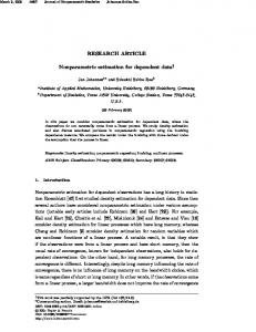
Fig. 1. 3dMDheadTM System with five camera units for imaging the whole head. There are three camera units in the front and the two units in the back cannot be seen in the picture. One camera unit includes a projector, two cameras to measure 3D data and one camera to record the texture of the skin. Two units can be taken along for mobile use to record facial 3D models. The white booth helps balance the lighting.
19
Fig. 2. Facial 3D surfaces and triangular polygons. Surface (A) includes 18 986 vertices and 37 531 faces and (B) includes 2 878 vertices and 5 624 faces.
stereophotogrammetry, the 3D coordinates of points on an object are measured from two or more photographic images taken from different positions. The 3dMDTM (Atlanta, Georgia, USA) camera system projects a radial grid onto a face or a head and then common points can be identified on each image. The 3D location of the points on the surface of the object is determined by triangulation based on the location and position of the cameras. Stereophotogrammetry provides a short acquisition time, which is a necessary feature when imaging very mobile infants and young children. Figure 1 shows the 3dMDheadTM System with five camera units. Generally, a digital 3D surface is reconstructed by connecting all the 3D points to form polygonal faces. Faces can consist of quadrilaterals or other simple convex polygons, but triangular faces are usually used, as in this work. The number of vertices and triangular faces in a craniofacial 3D surface can be tens of thousands, depending on the desired accuracy. Figure 2 shows a facial surface with two different triangulations. Usually, craniofacial 3D images are taken so that the nose points in the direction of the positive z-axis. The location of the axes and the origin can be determined in several ways (see Zhurov et al. 2010, Meyer-Marcotty et al. 2012). Figure 3 shows an example of a facial 3D image with the coordinate axes. 20
Fig. 3. Facial 3D model and coordinate axes. In this study the sagittal plane (yz-plane) is set to go through the middle of the superimposition of the original and the mirrored facial model. Definition of the coronal (xy-plane) and the transverse plane (xz-plane) can vary depending on whether the object is a facial or a cranial model.
2.1
Measurement errors
The 3dMDTM Imaging System has been verified to consistently record geometric accuracy within a root mean square error of less than 0.2 mm. The reproducibility of a neutral expression has been studied in Paper I and the accuracy of reproducing a neutral facial expression was 0.17 mm on average. Manually marked landmarks at specific geometric locations corresponding to human biological features are commonly used in analyses of facial and cranial structures. Landmarks are used in this thesis for pose standardization and size scaling. According to Toma et al. (2009), the accuracy 21
of landmark identification based on laser scanning, a technique less accurate than the method used in our study, ranged from 0.39 mm to 1.49 mm. 2.2
Ethical considerations
For the twin study of Paper I, performed for the most part in Kaunas, Lithuania, a statement of approval was provided by the local ethics board. The studies of Papers II– IV, performed at the Oulu University Hospital, were approved by the Ethics Committee of the Northern Ostrobothnia Hospital District. Data acquisition was painless and required a short time. Informed consent was gained from all subjects or their parents prior to the examinations. Anonymity of the subjects has been secured by coding their id data.
22
3
Recognition of twin zygosities based on facial 3D models
3.1
Statistical pattern recognition
Statistical comparisons of MZ and DZ twins based on facial 3D images have been made previously (Naini & Moss 2004, Djordjevic et al. 2013a), but in Paper I we wanted to study in particular how accurately it is possible to classify zygosity automatically. For this we used statistical pattern recognition methodology (Webb 1999, Holmström & Koistinen 2010). Pattern classification is a problem of identifying to which one of a set of mutually exclusive classes an object belongs. In the case of zygosity classification, the number of classes is two and we therefore assign MZ and DZ twins to class 1 and class 2, respectively. In pattern recognition, classification is made on the basis of features measured from an object. Let the true class of an object be J and let X be a vector that contains a number of relevant features measured from it. Now J and X can be regarded as a pair of random variables with a joint distribution and the problem is to use X to guess J. Two classifiers were tested, the first of which was very simple, based on a single scalar feature, with the discriminant function defined by t(x) = x − c,
(1)
where c is some central tendency measured from the training data. The second method tried was a quadratic classifier whose discriminant function is 1 1 x − µ 1 ) − (xx − µ 2 )T Σ−1 x − µ 2) t(xx) = (xx − µ 1 )T Σ−1 1 (x 2 (x 2 2 � � � � Σ2 ) det(Σ P1 1 − log − log , Σ 2 det(Σ 1 ) P2
(2)
where µ i and Σ i are estimated by the sample mean vector and the sample covariance matrix of the training data belonging to class i. Pi is the prior probability which is chosen to be 0.5 for both classes. The decision rule for both classifiers is: if t(xx) ≤ 0, then x is classified to MZ; if t(xx) > 0, then x is classified to DZ. 23
For good results, all available data were used for training the classifiers and, for classification error estimation, leave-one-out cross-validation (LOOCV) was used to avoid the problems caused by the dependence of testing and training data (Webb 1999). 3.2
Data processing and analysis
For this study, faces of 106 Lithuanian twin pairs of the same sex (46 male pairs and 60 female pairs) were recorded by a portable 3dMDfaceTM System in Kaunas, Lithuania in 2011–2013. The zygosity of each twin pair had been determined by a blinded DNA test. One male pair was excluded due to excessive facial hair. Classification analysis was carried out for the male and female pairs separately as well as all the twin pairs together. Distinct parts like hair were removed from images. The edges of the facial surfaces were removed so that the facial size was almost equal between twins. The position of the faces was standardized as described in Zhurov et al. (2010). To equalize the magnitude of differences in 3D surfaces, two scaling methods based on 21 manually identified facial landmarks (Farkas 1994) were used. The landmark coordinates for each twin were translated so that their centroid was the origin and then a landmark matrix with the translated coordinates as its rows was constructed. In the first scaling method, all twins were scaled to the average Frobenius norm calculated from landmark matrices (Dryden & Mardia 1998). In the second scaling method, one of the twins was scaled by the same factor, but the other twin was scaled by the same scale factor as the first one. In this way, the relative size difference of the faces of a twin pair did not change. Analyses were also carried out without scaling. After scaling, the faces of a twin pair were superimposed using a best fit algorithm. Three feature statistics were computed to characterize the differences between the twins. These were the average distance (mm), the standard deviation of distances (mm), and the percentage coincidence of distances within 0.5 mm tolerance. Three measures of central tendency were calculated for feature statistics in the case of classifier (1). These were the mean, the median, and the value separating the ordered feature data into two groups based on the proportion of MZ and DZ twins. A quadratic classifier (2) was tested using feature vectors consisting of all these three quantities and combinations of pairs of them as well as single scalar features. 3D images were processed with Rapidform2006 (INUS Technology, Inc., Seoul, Korea). Pose standardization, scaling, superimposition of facial surfaces, and computation of the statistics were automated with a set of in-house VBA (Visual Basic for 24
Table 1. Success rates (%) for 3D zygosity classification compared to DNA testing with classifier (1). Rates above 80% are shown in bold. Scaling 1 Feature
Males
Females
Scaling 2 All
Males
No scaling
Females
Mean as a measure of central tendency AD 82.22 81.67 84.76 86.67 83.33 SD 80.00 85.00 80.00 82.22 76.67 Coinc. 82.22 75.00 78.10 88.89 86.67 Median as a measure of central tendency AD 86.67 78.33 82.86 88.89 85.00 SD 86.67 78.33 81.90 86.67 81.67 Coinc. 77.78 75.00 77.14 88.89 85.00 DNA zygosity ratio as a measure of central tendency AD 86.67 81.67 84.76 86.67 83.33 SD 86.67 81.67 82.86 86.67 76.67 Coinc. 77.78 76.67 78.10 84.44 86.67
All
Males
Females
All
86.67 80.00 86.67
84.44 84.44 88.89
85.00 80.00 86.67
88.57 81.90 88.57
85.71 83.81 86.67
84.44 88.89 88.89
85.00 81.67 85.00
86.67 84.76 89.52
85.71 84.76 86.67
84.44 86.67 84.44
83.33 80.00 86.67
84.76 82.86 87.62
AD: average distance SD: standard deviation of distances Coinc.: percentage coincidence of distances within 0.5 mm tolerance Table 2. Success rates (%) for 3D zygosity classification compared to DNA testing with quadratic classifier (2). Rates above 80% are shown in bold. Scaling 1 Feature
Males Females
3 features 2 (AD & SD) 2 (AD & Coinc.) 2 (SD & Coinc.) 1 (AD) 1 (SD) 1 (Coinc.)
80.00 80.00 80.00 77.78 84.44 80.00 82.22
81.67 81.67 85.00 80.00 83.33 80.00 78.33
Scaling 2 All 80.95 82.86 82.86 80.95 85.71 80.00 79.05
Males Females 86.67 86.67 82.22 84.44 86.67 86.67 88.89
85.00 81.67 83.33 83.33 85.00 76.67 86.67
No scaling All 86.67 86.67 84.76 83.81 85.71 80.00 87.62
Males Females 84.44 82.22 86.67 86.67 86.67 84.44 88.89
83.33 83.33 83.33 85.00 85.00 80.00 90.00
All 85.71 86.67 85.71 86.67 86.67 82.86 87.62
AD: average distance SD: standard deviation of distances Coinc.: percentage coincidence of distances within 0.5 mm tolerance
Applications) subroutines developed for Rapidform. Statistical pattern recognition analyses were carried out using Matlab R2013b (MathWorks, Natick, Massachusetts, USA). 25
3.3
Success rates
There were three twin groups, three scaling methods, and three features to measure the difference between faces, and for classifier (1) there were three measures of central tendency to assign pairs to two classes. Features could be input in seven different ways for classifier (2), so there were 63 different classification scenarios altogether for classifier (2) and 81 for classifier (1). 3D classification was compared to DNA testing and the success rates are displayed in Tables 1 and 2. Success rates of at least 80% are shown in bold. In most cases the success rate was above 80%, so both classifiers provided relatively reliable zygosity recognition. Figure 4 shows examples of facial 3D images of falsely and correctly classified twin pairs. The first scaling method performed clearly worse than the other two, of which no scaling worked slightly better than the second scaling method. Including more than one component in the feature vector did not improve the performance of the quadratic classifier (2). The reason for this is probably the strong correlation between the features. Coincidence with 0.5 mm tolerance seems to be the most suitable feature with both classifiers when using the second scaling method or no scaling. When using these same scaling methods, the median was the best measure of central tendency for classifier (1).
Fig. 4. (A) Female DZ twin pair according to DNA but not 3D analysis. (B) Female MZ twin pair according to DNA but not 3D analysis. (C) Male MZ twin pair according to DNA and 3D analysis. (D) Male DZ twin pair according to DNA and 3D analysis (Paper I, published by permission of Cambridge University Press).
26
4
Analysis of head flatness and asymmetry using kernel density estimation on a sphere
Head shape analysis from cranial 3D images has been used in particular in studies dealing with infant head deformations. Typical syndromes are deformational plagiocephaly, which is characterized by an asymmetrical occipital flattening, and brachycephaly where flattening occurs across the whole occiput (Hutchison et al. 2004, Robinson & Proctor 2009, Laughlin et al. 2011). Asymmetry in craniofacial 3D images has been quantified for example by dividing the skull volume into four parts and then measuring ratios of volumes within these quadrants (Meyer-Marcotty et al. 2012). Lanche et al. (2007) defined the magnitude of asymmetry by the ratio of distances between the origin and the point on the head surface and the corresponding point on the other side of the sagittal plane (yz-plane). Atmosukarto et al. (2009, 2010) measured posterior skull flattening by using the distribution of head normal vector directions. The normal vector distribution was represented as a 2D histogram and asymmetry and flatness scores were measured using bin counts. Inspired by such an approach, we explored in Paper II the use of a smooth kernel density estimate of the directional data defined by the surface normal vectors to measure the asymmetry and flatness of the head. 4.1
Methods
4.1.1
Kernel density estimation on a sphere
Methods of directional statistics are described in Mardia (1972), Fisher et al. (1987). Silverman (1986), Wand & Jones (1994) are accessible introductions to kernel estimation methods in Euclidean space. Kernel density estimation on a sphere is described in Hall et al. (1987). Consider the unit sphere Sd = {xx ∈ Rd+1 | kxxk = 1} of the d + 1dimensional Euclidean space and a directional random vector X ∈ Sd with a density f . The kernel estimator of f based on a sample X 1 , . . . , X n ∼ f can be defined as � c(κ) n K κxxT X i , fˆ(xx; κ) = ∑ n i=1
x ∈ Sd ,
(3)
where K is a suitable kernel function and κ > 0 is the smoothing parameter. The normalization constant c(κ) is chosen so that the estimator integrates to unity. The 27
smoothing parameter can be written as 1/h2 to make the estimator more reminiscent of the Euclidean bivariate kernel density estimator � � x − Xi 1 n fˆ(xx; h) = 2 ∑ K , nh i=1 h
x ∈ R2 .
(4)
According to Hall et al. (1987), the kernel K in (3) should be a rapidly varying function such as the exponential. An increase of smoothing parameter κ leads to a rougher and more variable estimator. Let d = 2 and K(t) = et . Then the formula (3) becomes n T κ c(κ) n κxxT X i = e eκxx X i , fˆ(xx; κ) = ∑ ∑ n i=1 4nπ sinh(κ) i=1
x ∈ S2 .
(5)
The kernel density estimate (5) is in fact an arithmetic mean of von Mises-Fisher densities with different sample units as mean directions. The von Mises-Fisher distribution on S2 can be considered as the spherical counterpart of the circularly symmetric bivariate normal distribution. To choose the smoothing parameter value, we used the rule of thumb (ROT) suggested in García-Portugués (2013) � κROT =
ˆ + 4κˆ 2 ) sinh(2κ) ˆ − 2κˆ cosh(2κ)]n ˆ κ[(1 ˆ 8 sinh2 (κ)
�1/3 ,
(6)
where κˆ is the maximum likelihood estimate of the concentration parameter of the von Mises-Fisher density. Note that in the study of García-Portugués (2013), the ROT √ smoothing parameter was represented as hROT = 1/ κROT . ROT assumes that the estimated data follows the unimodal von Mises-Fisher distribution. Infant head data usually include more than one mode but ROT selection of the smoothing parameter worked well in our data analyses. 4.1.2
Visualization of the spherical kernel density estimate
Visualization of the spherical kernel density estimate is done by using a planar contour plot. The sphere is mapped onto the disk using the Lambert azimuthal equal area projection (see Fisher et al. 1987). As the name suggests, this projection maps equal areas on the sphere onto equal areas on the plane. In the Lambert projection the spherical coordinates (θ , ϕ) and the polar coordinates (ρ, ψ) are related by ρ = 2 sin((π − ϕ)/2) and ψ = θ , where 0 ≤ θ ≤ 2π and 0 ≤ ϕ ≤ π. Distortion in the projection increases 28
with distance from the center of the projection disk and therefore the shape of density in areas lying near the boundary of the disk can be difficult to interpret. As a remedy, the sphere can be divided into two hemispheres which can be projected onto two disks and √ then 0 ≤ ρ ≤ 2. However, since we examine the posterior side of the head, only one hemisphere is needed. Figure 5 shows an example of a projected contour plot and how flat areas can be highlighted in the 3D head by thresholding the density estimate. The infant of Figure 5A has plagiocephaly and an infant with brachycephaly is shown in Figure 5B. To draw contour plots in a computationally efficient manner, an equispaced grid on S2 is needed. It is not possible to construct a regular Cartesian grid on the sphere but the so-called Fibonacci grid offers a virtually equispaced mesh of points on S2 (see Swinbank & Purser 2006). Regular patterns seen in many plants and flowers can be characterized by Fibonacci numbers and this inspired the definition of the Fibonacci grid. Swinbank & Purser (2006) defined a set of basis vectors corresponding to grid intervals along the spirals of the Fibonacci grid. These vectors obey a recurrence relationship similar to Fibonacci numbers and therefore justifying the name “Fibonacci grid”. The grid points on the unit sphere are defined by the spherical coordinates θi = 2πiγ −1 ,
(7) �
ϕi =
π 2i − arcsin 2 2m + 1
� (8)
√ where γ = (1 + 5)/2 is the golden ratio and the points are indexed from −m to m. The contour plot is computed using the values of the density estimate at the projected Fibonacci grid points. Figure 6 shows an example of a Fibonacci grid with 3001 points (m = 1500). 4.1.3
Scores for measuring flatness and asymmetry
The head normal directions X 1 , . . . , X n ∈ S of the selected area from the cranial 3D image are thought to represent a sample from a density f : S → [0, ∞[ defined on the unit sphere. Spherical shape in the area of interest would make f the density of the uniform distribution on a subset S0 ⊂ S of the unit sphere. Therefore flat regions lead to local maxima in the density (Figure 7A and 7B) and this “roughness” in the shape of the density can be measured by the integral of its square (Scott (1992), Sec. 3.2.2). By Schwarz’s inequality, it can be shown that the roughness of f attains its minimum value 29
Fig. 5. Contour plot of a kernel density estimate of head unit normal directions projected onto the disk and the flat regions of the head located by thresholding the density estimate. The values of the azimuthal angle θ and the polar angle ϕ are marked on the circumference and in the interior of the disk, respectively. The color bar indicates the height of the density estimate. In the 3D image, colored regions flag triangular faces where the threshold was set at a specific portion of the maximum value of the density estimate. In the red, yellow and blue regions the threshold was for (A) 80%, 75%, and 70% and for (B) 95%, 75%, and 55%, respectively (Paper II, published by permission of Wiley).
for the uniform density. This motivated the use of the roughness of kernel estimate (5) Z
FS = 4π
fˆ(xx; κ)2 dS
(9)
S
as a flatness score. Due to the scaling factor of 4π, the score FS ≥ 1 and the higher the value of FS is, the more flatness occurs on the head. 30
Fig. 6. A Fibonacci grid of 3001 poins.
To measure asymmetry, we compared the whole head area of interest to its mirror image (Figure 7C). Thus, consider the estimator (5) and denote x = [x, y, z]T , X i = [Xi ,Yi , Zi ]T so that
c(κ) n κ(xXi +yYi +zZi ) fˆ(xx; κ) = . ∑e n i=1
Our proposal for the asymmetry score then is Z � �2 AS = fˆ(x, y, z; κ) − fˆ(−x, y, z; κ) dS.
(10)
(11)
S
This score measures the difference between the head unit normal distribution and its reflection across the yz-plane. Sometimes the back of the head can be very round and symmetrical, but at the same time it lies obliquely with respect to the face. We therefore propose to scale (11) by the 31
Fig. 7. (A) The surface normal vectors in the flat area have similar directions. (B) This leads to a local maximum in their distribution. (C) The difference of this distribution and its reflection indicates possible asymmetry.
absolute value of the x coordinate of the most posterior point of the head divided by the width of the head. Width normalizes the scaling factor, removing the effect of infant head growth with age. Thus, let H ⊂ R3 be the 3D head model and let [x0 , y0 , z0 ]T = arg min z. [x,y,z]T ∈H
Setting � w(H) = |x0 |/
� max x − min x , [x,y,z]T ∈H
[x,y,z]T ∈H
the weighted asymmetry score is wAS = w(H) · AS.
(12)
If AS is small but at the same time the back of the head is asymmetrical with respect to the face, the scaling factor w(H) increases wAS. 4.1.4
Numerical integration
Numerical integration is needed to compute scores (9) and (11). We generated the Fibonacci grid (cf. Section 4.1.2), calculating the integral using a 2D analog of the rectangle rule for 1D integrals. Thus, if g : S → R is an integrable function on the unit sphere and l is large, then Z S
32
g(xx)dS ≈
4π l
l
∑ g(xxi ),
i=1
(13)
where x 1 , . . . , x l are Fibonacci grid points. Accuracy was tested by integrating the kernel estimates of our example data sets over S and we concluded that for the value l = 20 001 used in our application, the result deviated from the correct value of 1 by less than 3 · 10−7 . Monte Carlo integration was also tested but it was computationally much more expensive. 4.1.5
Previous quantification methods
Atmosukarto et al. (2009) represented spherical coordinates of head surface normal vectors as a 2D histogram with a fixed number of bins. To measure flatness, they constructed a severity score, where the algorithm performs a clustering procedure for sorted histogram bins, whose counts are above a specified threshold. The algorithm returns clusters which represent potential flatness and the 2D histogram flatness score (HFS) is the sum of the squared bin counts, which are in the returned clusters, multiplied by the number of these bins. In the study of Atmosukarto et al. (2010), two separate flatness scores are computed for either side of the head by summing the histogram bins that correspond to the combination of specific spherical angles. Then the 2D histogram asymmetry score (HAS) is the absolute value of the difference of the right and left flatness scores. Meyer-Marcotty et al. (2012) introduced the posterior cranial asymmetry index (PCAI) and Aarnivala et al. (2015) made slight changes to it. In the newer version, the region of interest in their head position Pose 2 is divided into two parts by the sagittal plane (yz-plane) and the PCAI tells how many percent the volume of the larger part is bigger than the volume of the smaller one. In Paper II we referred to PCAI as VRAS (volume ratio asymmetry score). Still other scores are calculated on the measurement plane that is parallel to the transverse plane (xz-plane) and goes through the most posterior point on the occiput (Meyer-Marcotty et al. 2012). The oblique cranial length ratio (OCLR) is the ratio between the longest and shortest oblique transcranial diameter on the measurement plane multiplied by 100, where the diameters form an angle of 40 degrees with the z-axis (Aarnivala et al. 2015). The cephalic index (CI) is the maximum cranial width divided by the maximum cranial length on the measurement plane multiplied by 100.
33
Fig. 8. Head position standardization and regions for analysis: (A) Pose 1 and (B) Pose 2 (Paper II, published by permission of Wiley).
4.2
Data analysis
4.2.1
Processing of the 3D image data
Images were recorded using the 3dMDheadTM System (Atlanta, Georgia, USA). All 3D image processing was carried out with Rapidform2006 and in-house VBA subroutines developed for Rapidform. Irrelevant parts, such as the shoulders and neck, were removed from the images. Subjects wore a tight sock to cover the hair, but hair nevertheless caused little bumps on the sock, so these bumps were also removed using image processing. We considered two alternative methods for head position standardization, both based on the subject’s facial area. The first, referred to as Pose 1, was defined as in section 3.2 (Zhurov et al. 2010) and the second, referred to as Pose 2, was defined as described in study of Aarnivala et al. (2015). After pose standardization, the head regions considered in surface normal measurements were defined. Next, for both poses, the head regions considered in surface normal measurements were delineated by two planes. Detailed descriptions of the two poses can be found in Paper II. Figure 8 illustrates the measurement regions for each pose. To ease the computational load, we reduced the number of triangular faces covering the measurement regions to approximately 6000. A Rapidform algorithm was used 34
to improve the quality of the resulting coarser triangularization. Many of the image processing steps were automated with a set of VBA subroutines. 4.2.2
Material and study design
Our studies included 99 infants who were born at the Oulu University Hospital and were recruited at birth on preselected dates between February 2012 and December 2013. In a previous study (Aarnivala et al. 2015) these newborn infants were randomized into two groups at birth. The intervention group received parental counseling about the infant’s environment, positioning, and handling. Due to ethical reasons, this procedure was terminated when the infants were 3 months old. 3D images of the infants used in this thesis were recorded at the ages of 3, 6 and 12 months. Structured clinical examinations and parental interviews were performed at each visit. 92 of 99 infants were able to come each time and 97 came for the first two. Participants have also attended 3-year follow-up visits and subsequent visits will take place at 6 and 9 years. In Paper II we tested the scores (9), (11), and (12) on the images of three-month-old infants. We compared our asymmetry scoring results with the methods of Atmosukarto et al. (2010) and Meyer-Marcotty et al. (2012) and also with clinical ratings made by two medical doctors (MD1 and MD2). The clinical application of our method is reported in Paper III, which considers the development of positional cranial deformation and associated risk factors. 4.2.3
Comparison of quantification methods
By examining the 3D images, two medical experts performed the clinical classification based on the rates of Argenta Argenta (2004). Classification was done twice in order to test the reproducibility of the rating results. The average of all four clinical scores was also calculated for comparison tests. Based on ratings, our data included only a few cases of posterior brachycephaly and therefore comparison between flatness score (9) and the clinical ratings could not be done properly. Therefore, we modified the head data (the region of Pose 1) artificially and quantified it by FS and the method based on 2D histograms (2D histogram flatness score (HFS)) (Atmosukarto et al. 2009). For four infants with low FS and HFS results, five gradually smoothed head surfaces were generated by Rapidform software. Also, for two infants, a hole was cut in the 3D model
35
Table 3. Cohen’s kappa coefficients for intra-rater and inter-rater agreement in asymmetry classification of 99 infants at the age of 3 months. Cohen’s kappa coefficient MD1 T1 MD1 T2 MD2 T1 MD2 T2
MD1 T1
MD1 T2
MD2 T1
MD2 T2
1 0.59 0.42 0.36
0.59 1 0.36 0.39
0.42 0.36 1 0.58
0.36 0.39 0.58 1
MD: medical doctor, rater T: time
five times, each time cutting a larger hole in the current model and filling it with a planar surface. Results for scores of the modified data are shown in Figure 9. Using all 99 images of three-month-old infants, asymmetry scores ((11) and (12)) were compared with two earlier proposals and clinical ratings. PCAI data were available from the previous study Aarnivala et al. (2015) and we implemented the algorithm of Atmosukarto et al. (2010) to measure HAS. The asymmetry scores were calculated for the regions of both poses. In numerical integrations, the size of the Fibonacci grid was 20 001 points. The scoring algorithms and the data analyses were carried out using Matlab R2014b. The relationship of the clinical classifications and asymmetry scores was summarized using the Spearman’s rank correlation coefficient. The Cohen’s kappa coefficient (Cohen 1960) was used to indicate intra- and inter-rater agreement of clinical scores. Tables 3 and 4 display the Cohen’s kappa and the Spearman’s rank correlation coefficients. 4.2.4
The course of positional cranial deformation from 3 to 12 months of age
In Paper III we investigated the natural course of cranial asymmetry and shape from 3 to 12 months of age using cranial 3D images. We studied whether different factors related to environment, care, diet, and illness had an impact on late cranial deformation or whether they failed to recover from previous cranial deformation. The study sought to assess the longitudinal relationship between deformational plagiocephaly, limited neck range of motion, and positional preference. Means and standard deviations of the shape scores at each visit are shown in Table 5. In statistical analyses, the data consisted of several characteristics of participants and measurements for quantifying asymmetry and flatness. A Chi-square test (χ 2 ), indepen36
Fig. 9. Summary of the results for the flatness scores: (A) HFS and (B) FS. The score value is on the vertical axis and the horizontal axis indicates the degree of flatness, with 0 corresponding to the original head (Paper II, published by permission of Wiley).
37
Table 4. Spearman’s rank correlation coefficients between asymmetry scores based on 3D models and clinical ratings. Correlations above 0.7 are shown in bold. Spearman’s ρ wAS R1 wAS R2 AS R1 AS R2 HAS PCAI MD1 T1 MD1 T2 MD2 T1 MD2 T2 MDavg
wAS R1
wAS R2
AS R1
AS R2
HAS
PCAI
1 0.75 0.77 0.67 0.61 0.53 0.63 0.64 0.66 0.62 0.73
0.75 1 0.69 0.73 0.48 0.65 0.66 0.67 0.68 0.68 0.79
0.77 0.69 1 0.86 0.65 0.39 0.54 0.50 0.50 0.52 0.58
0.67 0.73 0.86 1 0.57 0.36 0.60 0.52 0.53 0.49 0.59
0.61 0.48 0.65 0.57 1 0.40 0.47 0.44 0.45 0.48 0.51
0.53 0.65 0.39 0.36 0.40 1 0.44 0.59 0.63 0.70 0.66
wAS: weighted asymmetry score AS: asymmetry score HAS: 2D histogram asymmetry score PCAI: posterior cranial asymmetry index MD: medical doctor, rater MDavg: average of all clinical scores R1: region from Pose 1 R2: region from Pose 2 T: time
dent samples and paired samples t-tests and logistic regression analyses were performed to investigate potential risk factors for deformational plagiocephaly developing after 3 months of age, as well as for failure to recover from it by 12 months of age. We used a linear mixed model (Laird & Ware 1982) to analyze the impact of different factors on the development of cranial asymmetry and flatness. OCLR, ACAI, wAS, CI, and FS were used as dependent variables and putative predictive variables as fixed effects in the models. Values of wAS were multiplied by 100 000 to remove leading zeros. Values of FS seem different in Paper III because they were computed without using the scaling factor of 4π. The value of the dependent variable at 3 months of age was chosen to be a fixed effect so our model had a repeated measures design with two time points. Therefore, the use of linear mixed models was reasonable. We used a backward stepwise strategy to select the fixed effects for the final models. The Bayesian Information Criterion (BIC) was used to test model quality and models with the lowest BIC values were selected as the final models (Schwarz 1978). The BIC values also 38
Table 5. Means and standard deviations (shown in parentheses) for the asymmetry and flatness scores. Shape score OCLR PCAI AS wAS CI FS
at 3 months
at 6 months
at 12 months
103.06 (2.80) 9.32 (8.80) 7.37 (5.46) 27.14 (47.83) 77.49 (3.51) 2.55 (0.20)
102.55 (2.38) 7.83 (7.29) 5.75 (3.90) 21.33 (28.76) 78.40 (3.70) 2.57 (0.18)
102.33 (1.97) 7.14 (6.42) 5.35 (3.33) 20.57 (26.26) 77.51 (3.47) 2.51 (0.17)
OCLR: oblique cranial length ratio PCAI: posterior cranial asymmetry index AS: asymmetry score wAS: weighted asymmetry score CI: cephalic index FS: flatness score
indicated that Compound Symmetry could be used as the covariance structure for all the models. The final models are shown in Table 6. Statistical analyses were carried out with SPSS (v. 22.0, IBM, Armonk, New York). 4.2.5
Results
Figure 9 shows that in a comparison of flatness quantification methods, FS (9) outperformed HFS in both tests. A reasonable score should increase monotonically as flatness increases, but for HFS this happens only in test 1 in the case of infant 1, while FS behaves as expected. The intra-rater agreement for the clinical asymmetry ratings was moderate but only fair between the raters (Table 3). In the four separate ratings, 70 or more of the 99 infants scored 0, so the comparisons with classifications would have been more informative if the scores had been distributed more evenly. As Table 4 shows, the wAS (12) had the highest Spearman’s correlation with three of the four clinical ratings and also with the average of the clinical scores (MDavg). PCAI showed higher correlation in MD2 T2 (2nd rater’s 2nd rating). The asymmetry scores AS (11) and wAS (12) outperformed the HAS in all cases. Use of a weight factor clearly improved the performance of our asymmetry scores. The means of each asymmetry-related score decreased as time passed (Table 5). Decrease of asymmetry was more substantial between the first and the second visit than 39
40
Fixed effects OCLR PCAI wAS CI Intercept 39.73 (25.84–53.62)3 44.53 (13.14–75.92)2 -67.10 (-150.69– -16.48) 8.88 (-0.23–17.98) Value of dependent variable at 3 months 0.60 (0.50–0.71)3 0.59 (0.49–0.69)3 0.35 (0.28–0.42)3 0.90 (0.78–1.02)3 Preventive counseling at birth 0.17 (-0.35–0.70) 0.11 (-1.45–1.68) -2.65 (-8.87–3.56) -0.39 (-1.19–0.40) Time -12.80 (-20.80– -4.81)2 1.29 (-0.80–3.39) -3.09 (-10.00–3.81) 0.03 (-0.60–0.65) Head circumference 0.044 (-0.14–0.23) -0.73 (-1.26– -0.21)2 Gestational age at birth -0.01 (-0.09–0.07) 0.34 (0.05–0.64)1 Positional preference (supine) at 3 months 1.39 (0.43–2.36)2 5.68 (-2.80–8.57)3 14.60 (2.53–26.67)1 Neck rotation, imbalance 2.42 (1.20–3.64)3 Time spent in carriers/bouncers/car seats -0.014 (-0.55–0.52) -0.06 (-2.03–1.91) Time spent prone on the floor -0.14 (-0.24– -0.03)2 Otitis media 0.40 (-0.15–0.96) 0.74 (-0.91–2.39) Slept exclusively supine until 3 months -0.15 (-0.68–0.37) 0.16 (-1.46–1.79) -6.99 (-13.81– -0.16)1 0.20 (-0.63–1.04) Primary sleeping position Supine -6.24 (-13.43–0.96) -0.07 (-0.61–0.46) Side -4.59 (-11.52–2.33) -0.21 (-0.73–0.32) Prone – – Interaction term: Time 0.28 (0.11–0.45)2 × head circumference Interaction term: Positional preference 2.53 (1.15–3.91)3 at 3 months × neck rotational imbalance OCLR: oblique cranial length ratio; PCAI: posterior cranial asymmetry index; wAS: weighted asymmetry score; CI: cephalic index; FS: flatness score 1 p < 0.05, 2 p < 0.01, 3 p < 0.001
-0.061 (-0.084– -0.038)3
FS 0.90 (0.60–1.21)3 0.63 (0.51–0.75)3
Table 6. Coefficient estimates and 95% confidence intervals (shown in parentheses) of fixed effects for linear mixed models of cranial shape variables. Coefficients with p-value less than 0.05 are shown in bold. Fixed effects include repeated measurements, unless stated otherwise.
between the second and the third visit. Actually, only OCLR continued to improve significantly (p < 0.05) between the second and the third visit. At the second visit there was an increase in both flatness scores, but the increase was statistically significant only for CI. The scores eventually recovered or improved at the third visit. Linear mixed models differed from each other between the asymmetry scores and the flatness scores (Table 6). Positional preference at 3 months of age was the only statistically significant fixed effect in all asymmetry scores along with the score of first visit.
41
42
5
A scale space approach for spherical density estimation
Present scale space theory was developed in computer vision research (Lindeberg 1994). In statistics, Chaudhuri and Marron applied scale space ideas to nonparametric function estimation (Chaudhuri & Marron 1999). The underlying idea in their SiZer methodology was to explore simultaneously a whole family of different smooths. This approach avoided the need to select an optimal level of smoothing and the ever-present problem of bias in nonparametric function estimation. Since then, statistical scale space methods have been developed in various directions (Holmström & Pasanen 2016). Recently, Oliveira et al. (2014) proposed a SiZer-like method for circular data, called CircSiZer that applied kernel estimation with the von Mises density as the kernel function. In Paper IV we describe SphereSiZer, a novel scale space technique for the analysis of spherical data. This approach is similar to the method of Godtliebsen et al. (2002), used for analyzing a bivariate density function on a plane, in which the salient features of the density function are discovered by finding the locations where the gradient of the density surface differs significantly from zero. 5.1
Significant features in the scale space
Let the scale space presentation of the density function f be { f (·; κ) | κ > 0}, where f (·; κ) is a smooth of f . The smooth f (·; κ) is estimated by (5), described in Section 4.1.1, and then we get the estimate for this representation. Calculating the gradients to explore the features can be complicated on S2 . Hall et al. (1987) proposed a convenient approach where prior to calculating the gradient, the domain of the function of interest is extended beyond the sphere. Thus, for x ∈ R3 \ {00}, let g(xx) = f (xx/kxxk) and c(κ) n κ(xx/kxxk)T X i . g(x ˆ x; κ) = fˆ(xx/kxxk; κ) = ∑e n i=1
(14)
Now ∇g(·; ˆ κ) can be used as a test statistic to discover the statistically significant features of f (·; κ). To test the hypothesis H0 : ∇g(xx; κ) = 0 43
against H1 : ∇g(xx; κ) 6= 0 we first estimate the quantile q for which ( � ) � 3 Di g(x ˆ x; κ) − Di g(xx; κ) 2 P ∑ < q = 1 − α, SD(Di g(x ˆ x; κ)) i=1 where Di is the ith partial derivative, SD denotes standard deviation and 1 − α is the confidence level. The gradient estimator ∇g(x ˆ x; κ) can be considered as a weighted average of the gradient of the kernel function at different locations and therefore its standard deviation can be estimated as in Chaudhuri & Marron (1999), ! n TX c(κ) x x κ(x /kx k) i c i g(x c SD(D ˆ x; κ)) = SD ∑ Di e n i=1 � T T c(κ) � = √ s Di eκ(xx/kxxk) X 1 , . . . , Di eκ(xx/kxxk) X n , n where s denotes the sample standard deviation. Now the null hypothesis is rejected if #2 " 3 Di g(x ˆ x; κ) (15) ∑ c ˆ x; κ)) ≥ q. i=1 SD(Di g(x Gradients for scale space inference were calculated at the Fibonacci grid points G = {xx1 , . . . , x l } (see Section 4.1.2) on S2 . Chaudhuri & Marron (1999) eliminated data that was too sparse by estimating the effective sample size (ESS), which in our case is taken to be ESS(xx, κ) =
∑ni=1 K(κxxT X i ) K(κ)
and inference will only be considered in Aκ = {xx : ESS(xx, κ) ≥ 5}. Therefore, for a fixed κ, inference is considered for the grid points of the set Hκ = G∩Aκ . Quantile approximation was done with a bootstrap-t technique (cf. Efron & Tibshirani 1993). In bootstrap-t, one uses sampling with replacement to generate bootstrap samples ∗b X ∗b X 1 , . . . , X n }. Let gˆ∗b be the {X 1 , . . . , X n }, b = 1, . . . , B from the original data set {X ∗b X ∗b kernel density estimate (5) based on the bootstrap sample {X 1 , . . . , X n } and let #2 " 3 Di gˆ∗b (xx; κ) − Di g(x ˆ x; κ) Zb (xx; κ) = ∑ , b = 1, . . . , B. (16) c i gˆ∗b (xx; κ)) SD(D i=1
44
Simultaneous inference is used in quantile approximation to guard against an excessive number of significant features in SphereSiZer maps. For a fixed κ, the appropriate quantile q for inference which is simultaneous over all locations is the empirical quantile of max Zb (xx; κ), b = 1, . . . , B, and the quantile that is simultaneous x∈Hκ
over both x and κ is the empirical quantile of max max Zb (xx; κ), b = 1, . . . , B. The κ∈K x ∈Hκ
performance of the bootstrap based quantiles were tested by simulation. A random sample generated under the null hypothesis (the uniform distribution) was analyzed with SphereSiZer. With inference simultaneous over x , the rejection probability did not exceed much the given nominal significance level. When inference was simultaneous over both x and κ, the null hypothesis was never rejected. Hence, this approximation method is very conservative and the false positives will be rare. 5.2
SphereSiZer maps
Visualization of the spherical kernel density estimate is carried out as in Section 4.1.2. Again, the Fibonacci grid is mapped onto a planar disk using the Lambert projection. For SphereSiZer maps, the sphere is divided into two hemispheres which are projected separately onto two disks. When all the data is located in just one hemisphere, only one projection disk is needed. Finally, the significant gradients are plotted on the contour plot of the kernel density estimate, visualized by green arrows whose relative lengths correspond to the actual gradient magnitudes. Figure 10 shows an example of a SphereSiZer map. We call a collection of several maps a SphereSiZer atlas. An example is shown in Figure 11. A convenient way to view a large number of SphereSiZer maps simultaneously is a movie. All SphereSiZer analyses were programmed in Matlab R2016b. 5.3
Examples
We first generated simulated spherical data from mixtures of von Mises-Fisher densities. In general, let f (x) = p1 f1 (x) + . . . + pm fm (x) be a mixture of density functions where the weights pi > 0 satisfy ∑m i=1 pi = 1. A random sample point from this mixture is produced by generating first an index i uniformly on {1, . . . , m} according to the probabilities {p1 , . . . , pm }, and then generating a point from fi .
45
Fig. 10. An artificial test density and SphereSiZer maps on a complete sphere. (A) A contour plot of the test density with the 200 random sample points used in SphereSiZer analysis. (B) A SphereSiZer map based on this random sample. The smoothing parameter κ = 25. Whiter shading indicates higher density values and green arrows show statistically significant gradients. (C) A map projected along the x-axis (θ = 0, ϕ = π/2).
46
The probability density function of von Mises-Fisher distribution is fvMF (xx; µ , κ) =
T κ eκxx µ , 4π sinh(κ)
x ∈ S2 ,
where µ is the directional mean and κ > 0 is the concentration parameter. Figure 10A shows the contour plot of the first test density, f (xx) = 0.5 fvMF (xx; µ 1 , κ1 ) + 0.5 fvMF (xx; µ 2 , κ2 ), where µ 1 = (7π/24, 4π/6), µ 2 = (π/2, 0), κ1 = 35 and κ2 = 20. A SphereSiZer map of smoothing level κ = 25 based on a sample of 200 directions from the test density is shown in Figure 10B. In all examples, the confidence level is 1 − α = 0.95, the quantiles are simultaneous over both x and κ, the bootstrap sample size B = 500 and the maximum of (16) was computed using an x -grid G of size 1001 and a κ-grid K of size 40. In this first example, the data points are scattered over the whole sphere so the map consists of two disks. The azimuth angle is marked on the circumference of the disks. The left side is the projection of the northern hemisphere viewed from the positive z-axis (ϕ = 0). The polar angle ϕ = 0 lies at the centre and the meridian ϕ = π/2 is represented by the boundary of the projection disk. The right-hand disk is the projection of the southern hemisphere from the direction of the negative z-axis (ϕ = π) and the polar angle π is now at the centre. The SphereSiZer maps of Figure 10 suggests that the underlying density has two local maxima. Features in the borderline of hemispheres, as in Figure 10B, can be difficult to interpret. It may therefore be useful to consider projections also from other directions, such as along the x- (θ = 0, ϕ = π/2) or y-axes (θ = π/2, ϕ = π/2). Figure 10C shows the SphereSiZer map of this sample when the projection is taken along the x-axis. Now the azimuth angles are marked inside the disks while the polar angle markings lie outside the disks. The test density of the second example is f (xx) = 0.4 fvMF (xx; µ 1 , κ1 ) + 0.4 fvMF (xx; µ 2 , κ2 ) + 0.2 fvMF (xx; µ 3 , κ3 ), where µ 1 = (8π/15, π/6), µ 2 = (14π/15, 5π/24), µ 3 = (5π/3, 7π/18), κ1 = 40, κ2 = 40 and κ3 = 30. All simulated data lie on the northern hemisphere and hence only one projection disk is used for each map. In Figure 11, the SphereSiZer atlas shows how the significant features change with scale. The size of the random sample is again 200. For κ = 26, the significant gradients clearly imply the presence of two adjacent peaks. For κ = 20, a few significant gradients hint at a third peak near θ = 5π/3, ϕ = π/2. 47
Fig. 11. The second simulated test density and a SphereSiZer atlas based on a random sample of size 200 on the northern hemisphere. (A) A contour plot of the test density with the 200 random sample points and SphereSiZer maps with the smoothing parameter value (B) κ = 26, (C) κ = 20 and (D) κ = 12.
Increasing the smoothing level to κ = 12 merges two adjacent peaks and makes the third peak more significant. In the third example, we analyzed infant head surface normal vectors. We chose for SphereSiZer analysis a 3D image of one three-month-old infant with cranial asymmetry 48
Fig. 12. SphereSiZer analysis of infant head normal vector data. (A) Contour plot of the kernel density estimate of the set of 6736 head normal vector directions measured from the infant’s head and the random sample points used in SphereSiZer analysis. The size of the random sample was 1000 of which 959 points lie on the hemisphere displayed in the figure. SphereSiZer maps, based on this random sample, are simultaneous over x and κ with the smoothing parameter value (B) κ = 35, (C) κ = 25, and (D) κ = 15.
detected in previous studies (see Papers II and III). Normal vectors from the surface 49
region of Pose 1 (Figure 8) were analyzed in the example. Rapidform2006 was used for all image processing in this example. Figure 12A shows the contour plot of a kernel density estimate of 6736 surface normal directions placed more or less uniformly on the posterior side of the infant’s head. The smoothing level used was κ = 43.61, obtained using the ROT formula (6). For computational analyses, such a set of normal vector directions is very large and it furthermore cannot be regarded as a true random sample. Therefore, we sampled 1000 directions (Figure 12A) from the kernel density estimate based on the original sample of 6736 directions and then, to test the performance of SphereSiZer, used this smaller set for making inferences about the underlying true density. The kernel density estimate (5) can be regarded as a mixture of densities so that sampling can be done as in the previous two examples. Figure 12 also shows an atlas of three SphereSiZer maps of the 1000 normal vector directions. From (B) to (D) the values of κ are 35, 25 and 15. The presence of two local maxima in the data gets moderately strong support in each map.
50
6
Discussion
6.1
Twin zygosity classification
In twin zygosity classification based on facial 3D models, the simple classifier (1) performed competitively compared to the quadratic classifier (2). Both classifiers performed well, as all unscaled approaches and almost all methods based on the second scaling method achieved at least an 80 percent success rate. The results could perhaps be improved by better feature statistics, more effective scaling methods, larger training data sets, or more restricted age distributions. Rates could never reach 100 percent because of the presence of outlier twin pairs in both the MZ and DZ groups. Thus, some of the DZ twins have very similar faces and faces of MZ pairs may differ substantially in shape. 3D classification can never surpass DNA testing in zygosity analysis, but it is much faster and cheaper and therefore it may be used, for example, in approximating zygosities in a large set of twin data. In further studies, different regions of faces could be compared separately (Djordjevic et al. 2013a). Analyzing some specific areas could improve results in zygosity classification compared to the use of the whole facial surface. Analysis of different facial areas of MZ twins might detect the effect of specific genes in different parts of the face. One future study could consider testing human capability to recognize zygosity from 3D images compared to 3D analysis and DNA testing. Based on the reported success rates, on average, male twin pairs produced better results than female pairs, although the male sample was smaller. This is due to the fact that masculine features are more distinct than feminine ones and differences are therefore more obvious in male pairs. Opposite-sex twin pairs may have reduced dimorphism in various traits, due to suspected prenatal hormonal interference between fetuses (Heikkinen et al. 2013). It would therefore be interesting to study, using 3D facial images, if male opposite-sex twins have more feminine facial features than MZ or DZ male twins or if female opposite-sex twins have more masculine features than other female twins.
51
6.2
Infant head shape analysis
The novel scoring methods for quantifying head flatness and asymmetry, based on probability density estimates of directional data of three-month-old infants’ heads, worked better than some recently proposed 3D techniques. These novel scoring methods are distortion-free and automatic, so they do not require user-specified parameters as scores based on 2D histogram do (Atmosukarto et al. 2009, 2010). When comparing the performance of flatness scores with digitally modified head data, the FS exhibited the kind of monotonic relationship with increased flatness one would expect from a reasonable score, while the histogram-based HFS did not. The means of FS values behaved similarly to CI means from 3 to 12 months of age even though the correlation between CI and FS was weak (Pearson’s r = 0.325). Note that CI is not an actual 3D measurement because it is calculated on a 2D measurement plane such as the OCLR asymmetry score. The asymmetry scores proposed in Paper II outperformed the existing methods in many cases, as indicated by Spearman’s rank correlation with clinical ratings. In particular, wAS performed well and the correlation between wAS for the Pose 2 measurement region and the average of the clinical ratings was quite strong (Spearman’s ρ = 0.79). Aarnivala et al. (2017) extended clinical classification by also rating 3D images of children taken at 6, 12 and 36 months of age. In this follow-up study of Paper III, Receiver Operating Characteristic (ROC) curves were created for OCLR, PCAI, and wAS scores in order both to compare their accuracy and to determine the optimal cut-off values for deformational plagiocephaly and clinical rates. The study suggested that the simple OCLR score consistently provided the best discrimination and most accurate classification. The Argenta visual rating scale used in Paper II and Aarnivala et al. (2017) was originally developed for quantifying cranial deformities in infants with previously diagnosed deformational plagiocephaly, contributing to the lower intra- and inter-rater agreement compared to previous studies. Clinical ratings were determined by examining only cranial 3D surfaces, and therefore using real heads might have altered the results. The OCLR performs well, quantifying asymmetry in a manner similar to the Argenta score. This does not mean that other asymmetry quantification methods lack merit. The means of asymmetry scores had a similar kind of trend based on 3D models recorded at the ages of 3, 6 and 12 months. However, in the linear mixed models, the explanatory variables describing the scores varied considerably between the asymmetry 52
scores. Aarnivala et al. (2017) noticed that, although wAS had relatively low correlation with OCLR and PCAI, it still performs almost as well as OCLR. Therefore, wAS probably captures a different aspect of cranial shape than OCLR and PCAI. Asymmetry scores that measure the flatness of the head may capture shape information hidden to other methods. The unweighted AS can also be useful even if it fared worse in comparisons. It measures the asymmetry of the occiput while the weight takes into account the asymmetry with respect to the face. The two scores can therefore provide partly complementary information about the shape of the head and one might consider using them together. Both the flatness score, FS and the asymmetry score, AS, described in Paper II, consider only the distribution of normal vectors, and not the actual locations of the normals on the head surface. Therefore, theoretically, these methods may lead to an erroneous assessment of head shape. However, such situations do not occur in the context of the kind of naturally appearing head deformities studied in this thesis. 6.3
Scale space method for spherical data
SphereSiZer, a novel scale space method for spherical density estimation, can be viewed as a generalization of both CircSiZer and the Significance in Scale Space methodology (cf Oliveira et al. 2014, Godtliebsen et al. 2002). Significant features in different levels of scale are displayed by an atlas of planar contour plots overlaid with statistically significant gradient vectors. A movie of maps serves as an effective means for exploring features underlying the data in multiple scales. The test examples with the 3D infant head data and simulated data demonstrated how SphereSiZer works in practice. A causality condition, meaning no spurious structure should be generated when going from a coarser to a finer scale, is generally required in scale space analyses (see Witkin 1983, Koenderink 1984). In the linear Euclidean case, the Gaussian is the sole kernel that satisfies causality, but even then only for 1D signals (Lindeberg 1994). Huckemann et al. (2016) introduced the causal-satisfying WiZer method, which uses the wrapped normal distribution as the kernel and also developed new axiomatics for scale spaces of circular data. Similar axiomatics for spherical scale space analyses is a challenging topic for future research. We suspect that, with the von Mises-Fisher kernel non-causality is likely to occur only in very small scales. Especially with simultaneous inference, SphereSiZer would probably be unlikely to flag such small scale features as significant. Another interesting direction for future work would be to consider the 53
possibility of replacing the bootstrap approach in the quantile approximation with a more accurate method. This could be something similar to the approach of Hannig & Marron (2006) based on extreme value theory of Gaussian processes. The SphereSiZer methodology can be readily generalized for higher dimensions. The main problem would be the visualization and interpretation of the results. However, finding useful multi-dimensional analogues of SphereSiZer atlases could be challenging. Visualization of the multivariate spherical density could perhaps be accomplished using the volume function defined by its level sets. The volume function is a mode isomorphic, one-dimensional description of the mode structure of a multivariate density (Klemelä 2009, Holmström et al. 2017) and it could perhaps be usefully extended for directional data. García-Portugués et al. (2013) described a kernel density estimation for directional-linear data, a mixture of multivariate directional and linear data. Such data can be thought to lie on a multi-dimensional cylindrical surface. Marzio et al. (2011) considered kernel density estimation on a torus. Based on these estimators, new statistical scale space methods could be developed for densities of directional-linear and torus data.
54
References Aarnivala H, Vuollo V, Harila V, Heikkinen T, Pirttiniemi P & Valkama AM (2015) Preventing deformational plagiocephaly through parent guidance: a randomized, controlled trial. European Journal of Pediatrics 174(9): 1197–1208. Aarnivala H, Vuollo V, Heikkinen T, Harila V, Holmström L, Pirttiniemi P & Valkama AM (2017) Accuracy of measurements used to quantify cranial asymmetry in deformational plagiocephaly. Journal of Cranio-Maxillofacial Surgery 45(8): 1349 – 1356. Argenta L (2004) Clinical Classification of Positional Plagiocephaly. Journal of Craniofacial Surgery 15(3): 151–165. Atmosukarto I, Shapiro LG, Cunningham ML & Speltz M (2009) Automatic 3D Shape Severity Quantification and Localization for Deformational Plagiocephaly. Proceedings of SPIE 7259(725952). Atmosukarto I, Shapiro LG, Starr JR, Heike CL, Collett B, Cunningham ML & Speltz ML (2010) 3D Head Shape Quantification for Infants with and without Deformational Plagiocephaly. The Cleft Palate-Craniofacial Journal 47(4): 368–377. Chaudhuri P & Marron JS (1999) SiZer for Exploration of Structures in Curves. Journal of the American Statistical Association 94(447): 807–823. Cohen J (1960) A Coefficient of Agreement for Nominal Scales. Educational and Psychological Measurement 20(1): 37–46. Collett BR, Heike CL, Atmosukarto I, Starr JR, Cunningham ML & Speltz ML (2012) Longitudinal, Three-Dimensional Analysis of Head Shape in Children with and without Deformational Plagiocephaly or Brachycephaly. The Journal of Pediatrics 160(4): 673 – 678.e1. Djordjevic J, Jadallah M, Zhurov AI, Toma AM & Richmond S (2013a) Three-dimensional analysis of facial shape and symmetry in twins using laser surface scanning. Orthodontics and Craniofacial Research 16(3): 146–160. Djordjevic J, Pirttiniemi P, Harila V, Heikkinen T, Toma AM, Zhurov AI & Richmond S (2013b) Three-dimensional longitudinal assessment of facial symmetry in adolescents. European Journal of Orthodontics 35(2): 143–151. Djordjevic J, Toma AM, Zhurov AI & Richmond S (2014) Three-dimensional quantification of facial symmetry in adolescents using laser surface scanning. European Journal of Orthodontics 36(2): 125–132. Dryden I & Mardia K (1998) Statistical Shape Analysis. Wiley series in probability and statistics. Wiley, Chichester, England. Efron B & Tibshirani R (1993) An Introduction to the Bootstrap. Chapman & Hall, New York. Farkas L (1994) Anthropometry of the head and face. Raven Press, New York. Fisher N, Lewis T & Embleton B (1987) Statistical Analysis of Spherical Data. Cambridge University Press, Cambridge, England. García-Portugués E, Crujeiras RM & González-Manteiga W (2013) Kernel density estimation for directional-linear data. Journal of Multivariate Analysis 121(Supplement C): 152 – 175. García-Portugués E (2013) Exact risk improvement of bandwidth selectors for kernel density estimation with directional data. Electronic Journal of Statistics 7: 1655–1685. Godtliebsen F, Marron JS & Chaudhuri P (2002) Significance in Scale Space for Bivariate Density Estimation. Journal of Computational and Graphical Statistics 11(1): 1–21.
55
Hall P, Watson GS & Cabrera J (1987) Kernel density estimation with spherical data. Biometrika 74(4): 751–762. Hannig J & Marron JS (2006) Advanced Distribution Theory for SiZer. Journal of the American Statistical Association 101(474): 484–499. Heikkinen T, Harila V, Tapanainen JS & Alvesalo L (2013) Masculinization of the Eruption Pattern of Permanent Mandibular Canines in Opposite Sex Twin Girls. American Journal of Physical Anthropology 151(4): 566–572. Holmström L & Koistinen P (2010) Pattern recognition. Wiley Interdisciplinary Reviews: Computational Statistics 2(4): 404–413. Holmström L, Karttunen K & Klemelä J (2017) Estimation of level set trees using adaptive partitions. Computational Statistics 32: 1139–1163. Holmström L & Pasanen L (2016) Statistical scale space methods. International Statistical Review DOI: 10.1111/insr.12155. Huckemann S, Kim KR, Munk A, Rehfeldt F, Sommerfeld M, Weickert J & Wollnik C (2016) The circular SiZer, inferred persistence of shape parameters and application to early stem cell differentiation. Bernoulli 22(4): 2113–2142. Hutchison BL, Hutchison LA, Thompson JM & Mitchell EA (2004) Plagiocephaly and Brachycephaly in the First Two Years of Life: A Prospective Cohort Study. Pediatrics 114(4): 970–980. Kau CH & Richmond S (2010) Three-Dimensional Imaging for Orthodontics and Maxillofacial Surgery. John Wiley & Sons, Ltd., Chichester, England. Klemelä J (2009) Smoothing of Multivariate Data: Density Estimation and Visualization. Wiley Series in Probability and Statistics. Wiley, Hoboken, NJ. Koenderink JJ (1984) The Structure of Images. Biological Cybernetics 50(5): 363–370. Laird NM & Ware JH (1982) Random-Effects Models for Longitudinal Data. Biometrics 38(4): 963–974. Lanche S, Darvann TA, Ólafsdóttir H, Hermann NV, Van Pelt AE, Govier D, Tenenbaum MJ, Naidoo S, Larsen P, Kreiborg S, Larsen R & Kane AA (2007) A Statistical Model of Head Asymmetry in Infants with Deformational Plagiocephaly. In: Ersboll B & Pedersen KS (eds) Image Analysis, volume 4522 of Lecture Notes in Computer Science, 898–907. Springer Berlin Heidelberg. Laughlin J, Luerssen TG & Dias MS (2011) Prevention and Management of Positional Skull Deformities in Infants. Pediatrics 128(6): 1236–1241. Lindeberg T (1994) Scale-Space Theory in Computer Vision. Kluwer Academic Publishers, Dordrecht, the Netherlands. Mardia K (1972) Statistics of Directional Data. Academic Press, London. Marzio MD, Panzera A & Taylor CC (2011) Kernel density estimation on the torus. Journal of Statistical Planning and Inference 141(6): 2156 – 2173. Meyer-Marcotty P, Böhm H, Linz C, Kochel J, Stellzig-Eisenhauer A & Schweitzer T (2014) Three-dimensional analysis of cranial growth from 6 to 12 months of age. European Journal of Orthodontics 36(5): 489–496. Meyer-Marcotty P, Böhm H, Linz C, Kunz F, Keil N, Stellzig-Eisenhauer A & Schweitzer T (2012) Head orthesis therapy in infants with unilateral positional plagiocephaly: an interdisciplinary approach to broadening the range of orthodontic treatment. Journal of Orofacial Orthopedics/Fortschritte der Kieferorthopädie 73(2): 151–165.
56
Naini FB & Moss JP (2004) Three-dimensional assessment of the relative contribution of genetics and environment to various facial parameters with the twin method. American Journal of Orthodontics and Dentofacial Orthopedics 126(6): 655 – 665. Oliveira M, Crujeiras R & Rodríguez-Casal A (2014) CircSiZer: an exploratory tool for circular data. Environmental and Ecological Statistics 21(1): 143–159. Riphagen JM, van Neck JW & van Adrichem LN (2008) 3D Surface Imaging in Medicine: A Review of Working Principles and Implications for Imaging the Unsedated Child. Journal of Craniofacial Surgery 19(2): 517–524. Robinson S & Proctor M (2009) Diagnosis and management of deformational plagiocephaly. Journal of Neurosurgery: Pediatrics 3(4): 284–295. Schwarz G (1978) Estimating the Dimension of a Model. The Annals of Statistics 6(2): 461–464. Scott DW (1992) Multivariate Density Estimation: Theory, Practice, and Visualization. John Wiley & Sons, Inc., New York. Silverman B (1986) Density Estimation for Statistics and Data Analysis. Chapman & Hall/CRC Monographs on Statistics & Applied Probability. Taylor & Francis. Swinbank R & Purser RJ (2006) Fibonacci grids: A novel approach to global modelling. Quarterly Journal of the Royal Meteorological Society 132(619): 1769–1793. Toma AM, Zhurov A, Playle R, Ong E & Richmond S (2009) Reproducibility of facial soft tissue landmarks on 3D laser-scanned facial images. Orthodontics and Craniofacial Research 12(1): 33–42. Wand P & Jones C (1994) Kernel Smoothing. Chapman & Hall, London. Webb A (1999) Statistical Pattern Recognition. Arnold, London. Witkin AP (1983) Scale-space filtering. In: Proceedings of the Eighth International Joint Conference on Artificial Intelligence - Volume 2, IJCAI’83, 1019–1022. Morgan Kaufmann Publishers Inc., San Francisco, CA, USA. Zhurov A, Richmond S, Kau CH & Toma A (2010) Averaging Facial Images. In: ThreeDimensional Imaging for Orthodontics and Maxillofacial Surgery, 126–144. John Wiley & Sons, Ltd., Chichester, England.
57
58
Original publications Vuollo V, Sidlauskas M, Sidlauskas A, Harila V, Salomskiene L, Zhurov A, Holmström L, Pirttiniemi P & Heikkinen T (2015) Comparing Facial 3D Analysis With DNA Testing to Determine Zygosities of Twins. Twin Research and Human Genetics 18(6): 306–313. II Vuollo V, Holmström L, Aarnivala H, Harila V, Heikkinen T, Pirttiniemi P & Valkama AM (2016) Analyzing infant head flatness and asymmetry using kernel density estimation of directional surface data from a craniofacial 3D model. Statistics in Medicine 35(26): 4891–4904. III Aarnivala H, Vuollo V, Harila V, Heikkinen T, Pirttiniemi P, Holmström L & Valkama AM (2016) The course of positional cranial deformation from 3 to 12 months of age and associated risk factors: a follow-up with 3D imaging. European Journal of Pediatrics 175(12): 1893–1903. IV Vuollo V & Holmström L (2018) A scale space approach for exploring structure in spherical data. Computational Statistics and Data Analysis. In press. I
Reprinted with permission from Cambridge University Press (I), Wiley (II) and Springer (III) Original publications are not included in the electronic version of the dissertation.
59
60
ACTA UNIVERSITATIS OULUENSIS SERIES D MEDICA
1441. Huhtaniska, Sanna (2018) The association between antipsychotic benzodiazepine use with brain morphology and its changes in schizophrenia
and
1442. Sundquist, Elias (2018) The role of tumor microenvironment on oral tongue cancer invasion and prognosis 1443. Keto, Jaana (2018) The middle-aged smoker in health care : primary health care use, cardiovascular risk factors, and physician’s help in quitting 1444. Tiisanoja, Antti (2018) Sedative load and oral health among community-dwelling older people 1445. Alaraudanjoki, Viivi (2018) Erosive tooth wear and associated factors in Northern Finland Birth Cohort 1966 1446. Sinikumpu, Suvi-Päivikki (2018) Skin diseases and their association with systemic diseases in the Northern Finland Birth Cohort 1966 1447. Nortunen, Simo (2018) Stability assessment of isolated lateral malleolar supination-external rotation-type ankle fractures 1448. Härönen, Heli (2018) Collagen XIII as a neuromuscular synapse organizer : roles of collagen XIII and its transmembrane form, and effects of shedding and overexpression in the neuromuscular system in mouse models 1449. Kajula, Outi (2018) Periytyvän rintasyöpäalttiusmutaation kantajamiesten hypoteettinen perinnöllisyysneuvontamalli
(BRCA1/2)
1450. Jurvelin, Heidi (2018) Transcranial bright light : the effect on human psychophysiology 1451. Järvimäki, Voitto (2018) Lumbar spine surgery, results and factors predicting outcome in working-aged patients 1452. Capra, Janne (2018) Differentiation and malignant transformation of epithelial cells : 3D cell culture models 1453. Panjan, Peter (2018) Innovative microbioreactors and microfluidic integrated biosensors for biopharmaceutical process control 1454. Saarela, Ulla (2018) Novel culture and organoid technologies to study mammalian kidney development 1455. Virtanen, Mari (2018) The development of ubiquitous 360° learning environment and its effects on students´ satisfaction and histotechnological knowledge
Book orders: Granum: Virtual book store http://granum.uta.fi/granum/
D 1456
OULU 2018
UNIVERSITY OF OUL U P.O. Box 8000 FI-90014 UNIVERSITY OF OULU FINLA ND
U N I V E R S I TAT I S
O U L U E N S I S
ACTA
A C TA
D 1456
ACTA
U N I V E R S I T AT I S O U L U E N S I S
Ville Vuollo
University Lecturer Santeri Palviainen
Postdoctoral research fellow Sanna Taskila
Professor Olli Vuolteenaho
University Lecturer Veli-Matti Ulvinen
Ville Vuollo
University Lecturer Tuomo Glumoff
3D IMAGING AND NONPARAMETRIC FUNCTION ESTIMATION METHODS FOR ANALYSIS OF INFANT CRANIAL SHAPE AND DETECTION OF TWIN ZYGOSITY
Planning Director Pertti Tikkanen
Professor Jari Juga
University Lecturer Anu Soikkeli
Professor Olli Vuolteenaho
Publications Editor Kirsti Nurkkala ISBN 978-952-62-1854-0 (Paperback) ISBN 978-952-62-1855-7 (PDF) ISSN 0355-3221 (Print) ISSN 1796-2234 (Online)
UNIVERSITY OF OULU GRADUATE SCHOOL; UNIVERSITY OF OULU, FACULTY OF MEDICINE; MEDICAL RESEARCH CENTER OULU; OULU UNIVERSITY HOSPITAL
D
MEDICA