Nonparametric estimation of the distribution function in ... - Project Euclid

Bayesian Analysis (2009)

4, Number 4, pp. 573–598

Nonparametric estimation of the distribution function in contingent valuation models David S. Leslie∗ , Robert Kohn† and Denzil G. Fiebig‡ Abstract. Contingent valuation models are used in Economics to value nonmarket goods and can be expressed as binary choice regression models with one of the regression coefficients fixed. A method for flexibly estimating the link function of such binary choice model is proposed by using a Dirichlet process mixture prior on the space of all latent variable distributions, instead of the more restricted distributions in earlier papers. The model is estimated using a novel MCMC sampling scheme that avoids the high autocorrelations in the iterates that usually arise when sampling latent variables that are mixtures. The method allows for variable selection and is illustrated using simulated and real data. Keywords: binary choice regression, Dirichlet process, latent variable, mixture model, variable selection

1

Introduction

Contingent valuation (CV) is an important stated preference method that is widely used to value non-market goods such as parks or medical facilities. A hypothetical market is constructed and respondents are asked how much they are willing to pay for the good. Implementation of a CV study requires two key issues to be resolved: the distributional assumption about willingness to pay, which is our focus, and the elicitation format. Several types of question formats have been developed, but the dichotomous choice request supported by Arrow et al. (1993) is preferred to open-ended questions. Thus, rather than ask “How much would you be prepared to pay in order to receive a given service?”, subjects are asked “Would you be prepared to pay a specified amount to receive the service?” For a comprehensive discussion of contingent valuation methods with special reference to applications in environmental economics see Carson and Hanemann (2005) while Diener et al. (1998) provide a survey of applications in health economics. Our article estimates a CV model flexibly by using a binary choice model which is expressed in terms of a latent variable regression similarly to Albert and Chib (1993), but assuming that one of the regression coefficients is known, and using a Dirichlet process mixture prior base distribution (Escobar and West 1995) over the set of all ∗ Department of Mathematics, University of Bristol, Bristol, UK, mailto:david.leslie@bristol. ac.uk † School of Economics, University of New South Wales, Sydney, Australia, mailto:r.kohn@unsw. edu.au ‡ School of Economics, University of New South Wales, Sydney, Australia, mailto:d.fiebig@unsw. edu.au

c 2009 International Society for Bayesian Analysis °

DOI:10.1214/09-BA421

574

Nonparametric estimation in contingent valuation models

density functions of the latent variables. This results in a binary choice model where the data determine the distribution of the latent variables and hence the link function. Our model is more general than models that assume a specific link function, such as probit and logit models which assume normal and logistic latent variables respectively. We show that predictions under the Dirichlet process mixture prior can be much more accurate than those obtained by choosing a specific link function. We fit the model using a new Markov chain Monte Carlo simulation method that generates the latent variables simultaneously with the allocation to components of the mixture model. This is more efficient than a straightforward generalisation of the sampling scheme of Albert and Chib (1993) and Leslie et al. (2007) that updates the latent variables conditional on all the other parameters and then updates all the other parameters conditional on the latent variables, which would result in significant autocorrelations. Similar inefficiencies are encountered by Holmes and Held (2006) in the context of simple probit regression, and by Handcock et al. (2007) when latent variables from a mixture distribution are used to investigate clustering in social networks. Since the standard MCMC schemes for Dirichlet process models already consider each observation in turn on each iteration of the sampling process, this new block-updating scheme adds negligibly to the computation time per iteration. The idea of generalising the probit model using a Dirichlet process prior is not new. However, previous work uses a location mixture of normal distributions (Erkanli et al. 1993; Mukhopadhyay and Gelfand 1997), which does not account for heavy tails, or a scale mixture of normal distributions (Geweke and Keane 1999; Basu and Mukhopadhyay 2000b), which does not accommodate bimodality or skewness. Basu and Mukhopadhyay (2000a) generalise their method to include mixtures of truncated normal distributions, but this still does not produce the fully general, and natural, prior over latent variable distributions achieved in our article. An advantage of using the full Dirichlet process mixture prior in our article is that it becomes straightforward to carry out variable selection as in Kohn et al. (2001) because the standard marginalisation of the unknown noise distribution (Ferguson 1973; Antoniak 1974) results in a normal mixture model, in which most parameters can be integrated out when the variable selection step is carried out. However, such a general formulation of the model results in identifiability problems. Previous articles resolve this issue by fixing some characteristic of the latent variable distribution. For example Newton et al. (1996) use a prior which fixes the median and range of the latent variable distribution, and while they use a hierarchical model to allow inference over these fixed characteristics it is not trivial to understand the resulting prior structure over distributions. In contrast we identify the model by fixing one of the regression coefficients which is automatic in contingent valuation models and allows us to maintain the full, and well-understood, Dirichlet process mixture prior which has dense support on the set of density functions on the real line (Lo 1984). An alternative fully non-parametric approach models the argument of a given link function as a general function of the covariates (see for example Wood and Kohn 1998;

D. S. Leslie, R. Kohn and D. G. Fiebig

575

Mallick et al. 2000). However, this approach usually requires a large number of observations and is restricted to having only a small number of covariates. It is also difficult to implement when the covariates are both discrete and continuous. In Section 6 we discuss how our approach can be used more generally in binary regression models and illustrate with an example.

2

The Dirichlet process probit model

Most models of binary choice that assume linear dependence on a set of regressors can be expressed as yi = x0i β + ²i , (1) di = I{yi >0} , where di is the binary response associated with regressors xi , yi is a latent variable, β is a vector of regression coefficients, and ²i is a random variable from some distribution. In all of the standard models of binary choice, some distribution is assumed for the ²i : in probit regression this distribution is the standard normal distribution and in logit regression it is the standard logistic distribution. In these cases, the model is identified by the choice of distribution of ²i , and in particular by normalising the variance of these distributions. Our article does not specify a parametric distribution for the ²i , and instead places a prior over essentially all possible density functions on the real line. This results in a very general model for binary choice where the regressors enter linearly; in particular, both logit and probit regression are supported by the model, as are binary regressions with skewed or bimodal distributions for ²i . The prior is the Dirichlet process mixture of normal distributions used by Escobar and West (1995) for density estimation, and by Leslie et al. (2007) in the context of heteroscedastic linear regression. This prior is defined hierarchically as ²i | µi , σi2 ∼ µi , σi2 | G ∼ G ∼

N (µi , σi2 ) G DP(αG0 )

(2)

where N (µ, σ 2 ) is a normal distribution with mean µ and variance σ 2 , and DP(αG0 ) is a Dirichlet process with parameter αG0 (Ferguson 1973). Lo (1984) shows that if the support of G0 is R × R+ (so that positive density is given to any valid values of µ and σ 2 ) then the closure of the support of this prior on the distribution of ²i is the set of all density functions on the real line; following Escobar and West (1995), we therefore define the base distribution by (µ, σ 2 ) ∼ G0 iff σ 2 ∼ IG(aσ , bσ ) and

µ | σ 2 ∼ N (m, τ 2 σ 2 ),

where IG(a, b) denotes an inverse gamma distribution with shape parameter a and scale b.

576

Nonparametric estimation in contingent valuation models

Clearly, if prior knowledge is available the parameters of this prior can be selected manually. However, following Leslie et al. (2007), we use hyperpriors with “generic” parameter settings: α ∼ Ga(2, 4), m ∼ N (0, n), τ 2 ∼ IG(2, 1), aσ = 2, bσ ∼ Ga(0.5, 1), where Ga(a, b) denotes a Gamma distribution with shape parameter a and scale 1/b, and n is the number of observations in the sample. This prior maintains the same structure as that employed by earlier papers, including those by Escobar and West (1995) and Leslie et al. (2007); an appropriate prior distribution over densities for density estimation is an appropriate prior for densities in other settings too. The prior for α controls the amount of departure from the (inverse gamma/normal) base distribution for the latent variables. Escobar and West (1995) observe that the parameters in the prior for α have a strong effect on inference about the number of components in the mixture model which results from the Dirichlet process, but have much less influence on the estimate of an unknown density. The prior for σ 2 means that all the σi2 have similar values, but the value is unspecified and has a diffuse prior with expected value 1. The prior for µ must be proper, since we are dealing with mixture models (Richardson and Green 1997), but as more observations become available it can be made more diffuse; this scaling is achieved by allowing the prior variance to depend on the number of observations n (see also the discussion on hierarchical centring at the end of this section). Finally, the prior for τ 2 is chosen to be fairly diffuse but with mean 1. We have found that the hyperparameter settings above, along with the flexible prior structure, are adequate for most data sets. However, we can consider a more refined approach where we first fit a logistic or probit regression to the data by maximum likelihood or Bayesian methods. Using this fit we can estimate the likely range for the error term and use that to form a prior for σ 2 . With such a general formulation for the distribution of the ²i there is an identification problem. The parameters of this binary model are only identified up to scale, and so some normalisation is needed (beyond that provided by the prior). In particular, for this model it is difficult to consider scale-free estimates, such as those obtained by dividing by the variance of the noise or by a particular regression parameter at each iteration of the MCMC scheme; in the former case the variance is not an appropriate quantity to use for such a general noise distribution, and in the latter it is quite possible that a variable may be selected out at a particular iteration of the scheme. The usual convention is to fix some characteristic of the distribution of the latent variables, such as the variance (probit, logit models) or the mean (Basu and Mukhopadhyay 2000b). Our approach retains the full Dirichlet process mixture prior for the latent variable distribution and identifies the model by fixing a regression coefficient, which is automatic for the contingent valuation model and may be useful more generally as discussed in section 6. The model can now be estimated by placing a noninformative prior on the regression coefficient. However, to carry out variable selection for the model it is necessary to place a weakly informative prior the regression coefficients β that are not fixed. This prior is

D. S. Leslie, R. Kohn and D. G. Fiebig

577

specified through a vector of indicator variables J , such that Ji = 1

↔

βi 6= 0.

We follow Kohn et al. (2001) and assume that the unconstrained Ji are independent with P(Ji = 1 | θ) = θ and with θ uniformly distributed on [0, 1]. Denoting by βJ the non-fixed components of β for which Ji = 1, the prior for β is completed by specifying 0 −1 βJ | J ∼ N (0, nπ ) 2 (XJ XJ )

where 0 denotes a vector of zeros of the appropriate length, n is the number of observations, and XJ denotes the matrix consisting of the columns of X for which Ji = 1. This is a special case of the prior used by Nott and Leonte (2004), in which the information content of the prior is the same as the information content of one observation; see Kass and Wasserman (1995). It is necessary to use a proper prior for variable selection, but desirable to use a prior which is reasonably noninformative. The unit information prior is used extensively in many applications and has worked well in our examples. However, it is straightforward to generalize our treatment to the class of priors considered by Liang et al. (2008) in the linear regression case. Note that we can specify the model with a fixed intercept and with µ ∼ N (0, τ 2 σ 2 ). However, the hierarchical centring used in our article is known to result in more efficient inference (Gelfand et al. 1995). Note that m in G0 therefore takes the place of the intercept term.

3

Inference

This section describes how to perform inference on the Dirichlet process probit model using MCMC to draw samples from the posterior distribution. It is well known (Ferguson 1973; Antoniak 1974) that the random distribution G can be integrated out, resulting in allocation of observations to components of a finite normal mixture model. The updates to this allocation to components can be made without conditioning on the parameters µi and σi2 , so that it is unnecessary to use reversible jump MCMC (Green 1995). Conditional on an allocation to components, we draw the σi2 followed by the other parameters of the model. More specifically, once G is integrated out, the Dirichlet process prior is effectively a prior on partitions S of the observations into groups, with all observations in one component of the partition having the same values of µ and σ 2 . Writing nj for the number of observations allocated to group j, and k(S) for the total number of groups in the partition S, the prior on partitions is Qk(S) αk(S) Γ(α) j=1 Γ(nj ) p(S | α) = , (3) Γ(α + n) where Γ is the gamma function. The prior on the values of µ ˜j and σ ˜j2 , the mean and variance of each observation allocated to component j, is the base distribution G0 . See Green and Richardson (2001) for details.

578

Nonparametric estimation in contingent valuation models

Therefore, conditional on the hyperparameters, we could write down a joint posterior distribution for the latent variables y = (yi )i=1,...,n , the regression coefficients β, the ˜ = partition S and the component means and variances, which we will denote by µ ˜ 2 = (˜ (˜ µj )j=1,...,k(S) and σ σj2 )j=1,...,k(S) . However, this full posterior distribution is complex and not particularly instructive, so instead we concentrate on the conditional distributions that are needed for MCMC sampling. A simple sampling scheme updates all model parameters except for the latent variables conditional on y, then updates y conditional on all the model parameters. Since the sampling of all variables other than y is identical to the sampling under a comparable linear regression model (Leslie et al. 2007) the additional coding effort is minimal in this case. However, as observed by Holmes and Held (2006), updating latent variables conditional on a set of parameters, then updating the parameters, can result in high autocorrelations in the sampled iterates. This is a particular problem in our model and that of Handcock et al. (2007), in which the latent variables are sampled from a mixture distribution. To illustrate this point, consider the case of well-separated components of the mixture distribution, as in the bimodal example of Section 4. We assume for simplicity that there are two components in the normal mixture model for the latent variables. For some observations it will be clear to which component of the mixture model the latent variable should be allocated. However for others (those for which the true mean function x0i β is far from zero, for example) there will be little information in the data to aid the allocation to components, and the latent variable should be allocated frequently to both components of the mixture. However, when one updates the latent variable yi conditional on the allocation to components of the mixture model, it is likely that the sampled yi will clearly be associated with the current cluster membership. Furthermore, when one updates the allocation to components of the mixture model the latent variable will be strongly associated with previous cluster membership and a switch of membership is highly unlikely. We see that cluster membership and latent variable can be highly correlated and therefore updating them independently can result in a highly inefficient sampler. Instead of this naive sampling scheme we introduce a new technique for sampling when latent variables come from mixture models. In this scheme we update the allocation variable si and the latent variable yi as a block, conditional on the other latent variables, denoted by y−i , and the partition of the other observations, denoted by S−i . We don’t explicitly write the conditioning on the covariates, β, and the hyperparameters in the following equations to simplify notation. First, note that p(si , yi | y−i , S−i , d) ∝ p(d | y, S)p(si , yi | y−i , S−i )

(4)

where si runs over components of the partition S−i and in addition a new component consisting only of observation i. Hence we can calculate p(si , yi | y−i , S−i ) without worrying about the truncation imposed on y by the observations d. Now

D. S. Leslie, R. Kohn and D. G. Fiebig

579

Z Z p(si , yi | µ ˜ si , σ ˜s2i , y−i , S−i ) ×

p(si , yi | y−i , S−i ) =

p(˜ µsi , σ ˜s2i | y−i , S−i ) d˜ µsi d˜ σs2i ,

(5)

σ ˜s2i

where µ ˜si and are the parameters of the normal distribution associated with component si . Since we are using the conjugate inverse gamma/normal prior for component parameters, and the conditional distribution of the parameters of component si does not depend on observations not currently allocated to component si , we have (as in MacEachern 1994) that à ! a bj j exp(−bj /˜ σj2 ) µ ˜j − mj 2 p(˜ µj , σ ˜j | y−i , S−i ) = φ , (6) σ ˜j2 /(nj + τ −2 ) Γ(aj )(˜ σj2 )aj +1 where φ denotes the standard normal density function, P

mj

rl +mτ −2 , −2 n−i j +τ

=

µ

1 2

P

bj

= bσ +

rl

= yl − x0l β,

aj = aσ + rl2 + m2 τ −2 −

n−i j 2 P ( rl −mτ −2 )2 −2 n−i j +τ

¶

with all summations taken over the set {l ∈ Sj , l 6= i}, and n−i j the number of elements in this set (in the case where si denotes a component containing only i, the summations and n−i j take the value 0). In other words, the mean and variance of component j follow an inverse gamma/normal distribution with parameters that depend on the prior, on the current value of β, and on the latent variables of the observations allocated to component j. Furthermore, p(si , yi | µ ˜ si , σ ˜s2i , y−i , S−i )

= p(si | µ ˜ si , σ ˜s2i , y−i , S−i )p(yi | µ ˜ si , σ ˜s2i , y−i , S) = p(si | S−i )p(yi | msi , asi , bsi )

(7)

and it is again a standard calculation to combine (5), (6) and (7) to see that ¡ ¢ −2 p(si , yi | y−i , S−i ) = p(si | S−i )t2asi yi − x0i β; msi , (1 + 1/(n−i ))bsi /asi si + τ

(8)

where tν (x; l, s2 ) is the density of the t distribution with shape parameter ν, mode l, and ν variance ν−2 s2 (if ν > 2) evaluated at x. The term p(si | S−i ) can easily be evaluated from (3). Finally, we can use (4) to show that p(si | d, y−i , S−i ) Z = p(si , yi | d, y−i , S−i ) dyi Z ¡ ¢ −2 ∝ p(si | S−i ) t2asi yi − x0i β; msi , (1 + 1/(n−i ))bsi /asi dyi si + τ I{yi >0} =di





= p(si | S−i )T2asi (−1)di +1 q

x0i β ((1 +

+ m si

1/(n−i si

+ τ −2 ))bsi /asi )



(9)

580

Nonparametric estimation in contingent valuation models

where Tν (x) is the cumulative distribution function of the standard t distribution with shape parameter ν evaluated at x. It also follows directly from these calculations that, conditional on si , yi is drawn from a truncated t distribution, with shape 2asi , mean msi + x0i β, and variance asi −2 ))bsi /asi . (1 + 1/(n−i si + τ asi − 2 In the sampling scheme, we therefore condition on β and the hyperparameters, and go through each observation in turn, using Gibbs sampling to reallocate the observation to a component then sample a new latent variable for that observation, conditional on the latent variables and allocations of the other observations. This avoids the problem of autocorrelation caused by sampling latent variables conditional on allocations, then allocations conditional on latent variables. Note that even in the naive scheme for this model (which updates all the latent variables conditional on the model parameters and allocation variables, then updates the allocation variables conditional on the latent variables and the model parameters) each observation must be reallocated in turn to a new component of the mixture, and this is the most computationally intensive part of the scheme. For the improved scheme we are faced with the same computational bottleneck, but have reduced the autocorrelation problem described above. In practice we find that the running speed for comparable numbers of iterations is similar for both the naive and improved schemes, but convergence to the stationary distribution is faster for the improved scheme. Sampling the indicator variables J and regression coefficients β, as well as the hyperparameters, conditional on the latent variables y and the partition S, is identical to the method used by Leslie et al. (2007). A brief description is in Appendix A; a full description is available from the authors on request. One particular point to note is that since, conditional on the partition S, the model is Gaussian, one can perform variable ˜ and βJ and updating J as in Chan selection by integrating out all the parameters µ et al. (2006).

4

Simulation study

This section uses simulated data to show that our method works for various different noise distributions, including normal and logistic distributions. We compare our method with an unconventional Bayesian probit model, identified by fixing the same regression coefficient as is used to identify the Dirichlet process probit model and estimating the variance parameter (instead of fixing the variance to 1 and estimating every regression coefficient). We find that assuming normality results in reasonable inference on the regression coefficients, but posterior predictive probabilities are incorrectly estimated. On the other hand, the flexible model introduced in Section 2 results both in inference on β under a model which supports the data generating process, and more accurate posterior predictive probabilities. Each of our four examples uses a 500 × 5 design matrix of independent standard

D. S. Leslie, R. Kohn and D. G. Fiebig

581

normal random variables. The true regression coefficients are (1, 0, −1, 0, 0)0 , so that only the first and third covariates are relevant. We generate di = I{x0i β+²i >0} ,

i = 1, . . . , 500

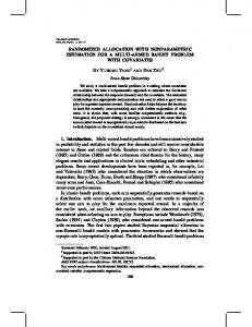
where ²i is distributed as: 1. a standard normal distribution, so that the probit model applies, 2. a logistic distribution, so that the logit model applies, 3. a mixture of two normal distributions, with weights 0.5, means of −2 and 2, and variance 0.25, and 4. log(Z) where Z is drawn from a χ22 distribution. Note that since the true value of β1 is 1, we identify the model by fixing β1 = 1; inference about the true generating distribution follows. In each case we ran the sampler for 11000 iterations, discarding the first 1000 for burn-in. For the full model, this took approximately 10 minutes in Matlab 7 on an Opteron 2GHz CPU, reducing to just 25 seconds when normality is assumed. We note that the reported results change very little if we take only 2000 observations in the sampling period. Furthermore, trace plots of the iterates of the parameters show no sign that the Markov chain has not converged to the stationary distribution. In all cases the correct variables are included in the model, and approximately correct posterior mean values for β are recovered. Inference for β is similar under both the restricted model and the general model. Table 1 shows the results. The most apparent differences between the models are observed in the estimated densities for the latent noise distributions, and the plots of predicted probabilities of observing a 1 at each set of covariates, shown in Figure 1. The clearest contrast between the normal distribution and the more flexible distribution occurs when the distribution is bimodal. The predictive probabilities are roughly equivalent to the ghosting approach of Marshall and Spiegelhalter (2003), also used by Leslie et al. (2007): we estimate pˆi = rep rep p(di = 1 | d) for each i = 1, . . . , n, where di is a replicated “ghost” of observation rep di with the same covariates, but independent latent noise ²i . More specifically, the estimate is given by pˆi ≈ (N − b)

−1

N X

rep p(di = 1 | d, β (t) , S (t) , θ(t) ),

(10)

t=b+1

where b gives the burn-in period, β (t) and S (t) are the sampled regression parameters and partition at iteration t, and θ(t) denotes the vector of all hyperparameters at iteration t. We see that

582

Nonparametric estimation in contingent valuation models

Table 1: Summaries of the posterior in the simulated experiments. The posterior mean of J and β are given for each experiment, with the posterior standard deviation of β given in brackets. Note that the posterior mean of J is the posterior probability of inclusion of the regression coefficients. Model: Variable x1 x2 Normal x3 x4 x5 x1 x2 Logistic x3 x4 x5 x1 x2 Bimod x3 x4 x5 x1 x2 Skew x3 x4 x5 Dataset

Normal probit J β 1.0000 1.0000(0.0000) 0.0412 0.0009(0.0143) 1.0000 −1.1262(0.1111) 0.0588 0.0045(0.0241) 0.0616 0.0053(0.0284) 1.0000 1.0000(0.0000) 0.1769 0.0243(0.0659) 1.0000 −0.8449(0.1231) 0.1091 −0.0093(0.0405) 0.0816 0.0027(0.0282) 1.0000 1.0000(0.0000) 0.1730 −0.0269(0.1115) 0.9999 −1.0018(0.2821) 0.1412 0.0108(0.0881) 0.1441 −0.0017(0.0851) 1.0000 1.0000(0.0000) 0.0545 −0.0032(0.0228) 1.0000 −0.9542(0.1041) 0.0513 −0.0029(0.0210) 0.1079 −0.0116(0.0425)

Dirichlet process probit J β 1.0000 1.0000(0.0000) 0.0339 0.0003(0.0129) 1.0000 −1.1251(0.1090) 0.0748 0.0055(0.0286) 0.0599 0.0043(0.0248) 1.0000 1.0000(0.0000) 0.1539 0.0214(0.0622) 1.0000 −0.8424(0.1265) 0.0688 −0.0054(0.0313) 0.0670 0.0022(0.0264) 1.0000 1.0000(0.0000) 0.1177 −0.0080(0.0485) 1.0000 −1.2507(0.1992) 0.1202 −0.0104(0.0509) 0.0748 0.0005(0.0344) 1.0000 1.0000(0.0000) 0.0555 −0.0034(0.0224) 1.0000 −0.9826(0.1091) 0.0625 −0.0033(0.0211) 0.0710 −0.0060(0.0317)

D. S. Leslie, R. Kohn and D. G. Fiebig Density estimates

583

Predictions assuming normality 1

Normal

0.5

0 −5

0

5

0.4 Logistic

0 −10

0

10

0.4 Bimodal

0 −10

0

10

0.4 Skew

0 −10

−5

0

5

0

Predictions under DP model 1 0.5

0

0.5

1

0

1

1

0.5

0.5

0

0

0.5

1

0

1

1

0.5

0.5

0

0

0.5

1

0

1

1

0.5

0.5

0

0

0.5

1

0

0

0.5

1

0

0.5

1

0

0.5

1

0

0.5

1

Figure 1: Posterior mean densities and predicted probabilities for the simulated results. In each case the true density (dotted), the estimated density assuming normality (solid), and the estimated density under a Dirichlet process prior (dashed) are shown in the left hand plot. Scatter plots of estimated probabilities against true probabilities are shown in the middle and right hand plots of each row.

rep p(di = 1 | d, β, S, θ)

rep = p(x0i β + ²i > 0 | d, S, θ)   k 0 X nj xi β + mj  = T2aj  q n + α −2 ))b /a (1 + 1/(n−i + τ j=1 j j j à ! 0 α xi β + m + T2aσ p n+α (1 + τ 2 )bσ /aσ

where nj , mj , aj and bj are as in (9) but without observation i removed. Figure 1 shows that the predictions can be quite different when the assumption of normality is dropped. In the experiment where the data are generated from a probit model, the analysis

584

Nonparametric estimation in contingent valuation models

under the general model results in near identical results to analysis under the normality assumption. In the case of bimodal or skewed noise, however, the density predictions are significantly different under the two analyses, with the general model resulting in accurate reporting of the generating density. The predicted probabilities under the general model are close to the true probabilities, whereas the normality assumption results in inaccurate predictions.

5

Contingent valuation

Responses in contingent valuation using a dichotomous choice format are binary, with di = 1 if subject i is offered a bid of bi and chooses to accept; otherwise di = 0. In this case, we know that subject i’s willingness to pay is greater than bi ; if we assume that the willingness to pay is of the form x0i β + ²i , where xi is a set of regressors associated with subject i, then di = 1

⇔

bi < x0i β + ²i .

Defining yi = −bi + x0i β + ²i = (bi

x0i )

µ ¶ −1 + ²i β

we see that di = I{yi >0} , and we have precisely the latent variable formulation (1). It is therefore natural to identify this model through fixing a coefficient instead of some characteristic of the latent variable distribution: the coefficient of bi is −1 through the formulation of the problem. In contrast with this, the standard method for analysing such data is to assume a parametric distribution for ²i , usually either a standard normal or logistic distribution (see for example Cameron and James 1987; Cameron 1988), then post-process the results to recover a coefficient of −1 for bi . Fern´andez et al. (2004) study a more complex contingent valuation model using Bayesian methodology, but their continuous noise terms are restricted to be skew-normal distributions. Our formulation can easily be extended to include the positive probability of having willingness to pay of 0 that is allowed under the model of Fern´andez et al. (2004), but we retain the simple probit structure to illustrate the differences between our flexible model and that originally used to study our data.

5.1

Contingent valuation of screening in rural Australia

We take the data from Clarke (2000) and analyse them using the method described in this paper, as well as under a normal Bayesian probit model with variable selection. The data consist of 372 responses to a survey of women in rural Australia, designed to assess the willingness to pay for visits of a mobile mammographic screening unit. See Clarke (2000) for a more complete description of the data including variable definitions. We first scaled all explanatory variables to have mean 0 and variance 1, to ensure that numerical

D. S. Leslie, R. Kohn and D. G. Fiebig

585

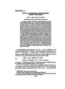
considerations do not affect the inference — without this rescaling the explanatory variables had variances ranging from 0.08 to 7586. The procedure outlined in Section 3 was then carried out, with β1 fixed to −1, before the results were transformed back to the original scale for reporting. Table 2 gives the posterior probabilities of inclusion, and the posterior means and standard deviations of the regression coefficients. Figure 2 plots the posterior density of the ²i . Table 2 shows that both estimation techniques result in probable inclusion of the “Intended use” variable, but not the “Distance” variable found to be significant (after various transformations) by Clarke (2000). When the error term is assumed normal, the marginal posterior probability of “Age” entering the regression is 0.25, but with the more general model for the errors the corresponding posterior probability is negligible. Furthermore, Figure 2 shows that the general model gives a very different prediction of the actual distribution of willingness to pay, with significant skewness of the distribution of ²i . To help compare these two models we consider the quantity X di =1

log pˆi +

X

log(1 − pˆi )

di =0

for each model, which is equivalent to comparing the deviances of each model. For the probit model this takes the value −209.4, whereas under the more general model it takes a value −198.7, which suggests that the Dirichlet process model fits the data more accurately. Although not reported here, we also ran the same procedures with the “Bid” variable transformed as in Clarke (2000). With this transformation, his simple variable selection procedure selected “Distance” as a significant variable. The full Bayesian methodology presented here contradicts this finding, both when normality is assumed and when it is not. The same variables are selected for the transformed data as for the untransformed data, and the estimated density for ²i remains highly skewed when normality is not assumed, despite the fact that the Box–Cox method is used to select the transformation of the “Bid” variable.

6

More general applications

We believe that our method can be used more generally because in many applications we would know, or expect, that some covariates should be in the regression with the sign of their coefficients known and the coefficient estimates highly statistically significant. A more general use of our method is now illustrated when the values (and signs) of the regression coefficients in a binary choice model are unknown, but we attempt to identify a suitable candidate coefficient to fix through a preliminary analysis of the data. In many econometrics problems the coefficient of price is a suitable candidate as it will be negative and significant. However, the method needs to be used with some caution as a suitable coefficient may be unavailable.

586

Nonparametric estimation in contingent valuation models

Table 2: Summaries of the posterior for the contingent valuation data. The posterior mean of J and β are given for each experiment, with the posterior standard deviation of β given in brackets. The covariates have the following meaning: Bid is the bid offered; Distance is the distance to the nearest fixed site (km); Intended use equals one if the respondent stated she would use a mobile unit if it visited their nearest town, otherwise 0; Married equals one if respondent is married; Senior high school equals one if respondent’s highest level of education is senior high school; Technical college equals one if respondent’s highest level of education is technical college; University equals one if respondent’s highest level of education is university; Age is respondent’s age (years); Knowledge equals one if respondent knows someone who has had breast cancer in the last five years; CART (Cancer Action in Rural Towns) equals one if the respondent lives in a CART intervention town; Received information equals one if the respondent stated that they had received the information sheet. Model: Normal Dirichlet process Variable J β J β Bid 1.0000 −1.0000(0.0000) 1.0000 −1.0000(0.0000) Distance 0.0989 0.0243(0.0846) 0.0729 0.0112(0.0473) Intended use 0.3104 19.7062(32.5992) 0.9495 71.2288(37.7568) Married 0.1004 4.1725(14.1757) 0.0709 1.6306(7.2644) Senior high school 0.0231 0.3870(5.5586) 0.0182 0.0359(2.6102) Technical college 0.0400 1.5015(9.9586) 0.0502 1.5125(7.8194) University 0.0299 0.9491(8.2568) 0.0218 0.4492(4.2909) Age 0.2753 −0.7093(1.2806) 0.0392 −0.0508(0.3083) Knowledge 0.0384 0.8878(5.7402) 0.0153 0.1863(2.2815) CART 0.0603 1.8374(8.6944) 0.0222 0.3250(2.9986) Received information 0.0250 −0.3701(5.7823) 0.0158 −0.2869(3.3314)

D. S. Leslie, R. Kohn and D. G. Fiebig

587

−3

5

x 10

4.5 4 3.5

Density

3 2.5 2 1.5 1 0.5 0 −1000

−500

0

500 ε

1000

1500

2000

Figure 2: Posterior mean density for ²i for the data of Clarke (2000). The estimates under normality and under the general model are given by the solid and dashed lines respectively.

6.1

PAP test awareness data

We reanalyse the data of Belkar et al. (2006) who consider whether Australian women are aware of the availability of a PAP smear test for the early detection of cancer of the cervix. Because the large majority of women in the sample are aware, this is an example of an unbalanced binary response and is one of the situations where traditional logit and probit models potentially give very different predictions. For our particular analysis, the other distinctive feature of this example is that, unlike the contingent valuation case, there is no clear candidate regressor on which to identify the model. However, by performing an initial analysis using a traditional probit model we select an identifying variable, then refine the initial analysis using the full model. The data consist of 8969 observations, which take value 1 if the subject is aware of the availability of PAP smear testing; 95% of subjects were aware of testing. The 29 explanatory variables consist largely of indicator variables, taking values one or zero depending on where survey respondents were born, where they live, their level of education, and their ability to speak English. In addition to these indicators, there are three variables which are also surveyed as ordered factors, but that we code as continuous values: age, income and spouse’s income, with the midpoint of the class taken as the response value. There are missing values for the two income variables, which are handled by retaining the data with missing observations and using the modified zero order method. If z has a missing observation it is coded as zero and a new dummy variable is created (zmiss) that equals 1 when the z observation is missing and is zero otherwise. The estimated coefficient on this dummy represents the estimated z effect for the missing observation. Finally, the square of each continuous variable was added

588

Nonparametric estimation in contingent valuation models

to the regression matrix. This dataset is fully described in Belkar et al. (2006). The results of a frequentist probit analysis are given in the first two columns of Table 3. We place the variable AGE2 first in the list, since this variable has the lowest p value, and is therefore an appropriate variable for fixing the regression coefficient; for the Bayesian approaches we identify the model by fixing this value to -1, and do not allow the variable to be selected out. We therefore scale the results of this initial analysis so that the first coefficient is −1, thus allowing easier comparison of the frequentist probit with the Bayesian methods presented here. Again, the variables were scaled to have mean 0 and variance 1, then the Bayesian procedures were run, before the results were rescaled to be reported on the original scale. For this more complex dataset we ran the sampler for 25000 iterations, discarding the first 5000 as burn-in. The programs in this case took approximately 25 minutes when normality was assumed, and 4400 minutes for the full model. Note that the time per iteration increases approximately linearly with the number of observations, since on each iteration we consider re-allocating each observation in turn to components of the mixture, so that these times are significantly longer than the previous examples because of the large amount of data. Table 3 gives the results of the frequentist analysis and the Bayesian analyses assuming both normal and general error distributions. Figure 3 shows the density estimates and the predicted probabilities, the latter analogous to those shown in Figure 1. These results show that the Dirichlet process does not show a large deviation from normality. Also shown in Figure 3 is a plot of predicted probabilities of awareness for women of different ages, comparing the difference in probability between Australian born and Asian born women of different ages. Table 3 shows being Asian born (ASBORN) is highly statistically significant, but that this translates into only small probability differences for the representative cases displayed in Figure 3. For this dataset, a logit regression results in different predictions to a probit regression. To test whether our method recognises data generated from a logit model, we use the posterior mean regression coefficients βˆ from the Bayesian probit analysis (column 5 of Table 3) to generate a second data set from the original design matrix. The logit noise terms were drawn from a logistic distribution then multiplied by 1/|βˆ1 |, where βˆlogit is the coefficient vector estimated by a logit analysis, so that the scale of the noise is approximately correct given the regression coefficients. The simulated observations d were then calculated, with 8657 of them being 1, a comparable number to those in the initial dataset. The same analyses as for the real data-set were applied. Figure 4 shows the density estimates and estimated probabilities. It is clearly seen that for this generated data set our model recognises the non-normal model, estimating heavier tails on the distribution of ²i than under the probit analysis. Furthermore, the predictions from the general model are more accurate than those from the restricted model, with the probit model consistently overestimating the lower probabilities (the distinct lines in the middle plot of Figure 4 are due to the mis-estimation of a regression coefficient corresponding to an indicator variable).

D. S. Leslie, R. Kohn and D. G. Fiebig

589

Table 3: Analysis of the PAP test awareness data.

Variable AGE2 AGE EXENG ENGLISH ENGEXENG NUBORN SEBORN WEBORN ASBORN OTBORN TERT DIPLOMA TRADE INC INC2 INCMISS SINC SINC2 SINCMISS VIC SA WA TAS NT ACT BRISBANE OTQLD RURAL REMRURAL

Frequentist probit Bayesian probit β p val J β −1.00 0.00 1.00 −1.00 (0.00) 91.18 0.00 1.00 90.74 (1.52) 631.65 0.00 1.00 662.82(113.11) 773.85 0.00 1.00 708.18(112.63) −195.05 0.36 0.01 −1.43 (25.50) 111.40 0.31 0.01 1.35 (17.46) −310.74 0.02 0.11 −36.18(110.50) 177.23 0.43 0.01 3.17 (38.34) −782.06 0.00 1.00 −698.60(113.20) 21.14 0.88 0.01 1.60 (22.91) 228.42 0.04 0.17 49.24(119.74) −26.26 0.80 0.01 −0.10 (6.53) 53.16 0.51 0.01 0.57 (10.75) 3.69 0.59 0.01 0.05 (0.57) 0.04 0.81 0.05 0.01 (0.03) 69.32 0.56 0.01 1.84 (19.53) 19.80 0.00 1.00 11.31 (2.54) −0.16 0.06 0.01 −0.00 (0.02) 338.30 0.01 0.12 36.88(107.88) −29.42 0.72 0.01 −0.35 (6.28) 139.62 0.16 0.03 4.61 (30.80) −132.25 0.21 0.02 −2.95 (23.18) −3.74 0.98 0.01 0.15 (11.84) −223.49 0.07 0.02 −3.40 (29.75) 114.28 0.36 0.01 2.45 (24.39) 103.85 0.49 0.01 1.36 (21.07) 122.33 0.45 0.01 0.89 (19.53) 84.93 0.49 0.00 0.41 (8.89) −36.12 0.69 0.01 −0.33 (8.48)

Dirichlet process J β 1.00 −1.00 (0.00) 1.00 90.63 (1.58) 1.00 691.85(125.21) 1.00 711.70(116.77) 0.01 −1.84 (29.50) 0.01 0.48 (9.05) 0.10 −34.94(110.87) 0.01 4.63 (52.89) 1.00 −710.71(118.89) 0.00 0.34 (10.23) 0.14 40.70(107.99) 0.00 −0.23 (7.56) 0.01 0.72 (11.68) 0.01 0.01 (0.26) 0.01 0.00 (0.01) 0.01 1.61 (17.24) 1.00 11.13 (2.61) 0.00 −0.00 (0.00) 0.13 42.75(118.70) 0.01 −0.60 (8.32) 0.02 2.62 (21.52) 0.01 −1.95 (19.31) 0.01 −0.40 (10.52) 0.02 −3.84 (30.46) 0.01 2.15 (22.91) 0.00 0.28 (9.42) 0.00 0.19 (8.55) 0.00 0.41 (10.92) 0.01 −0.13 (7.37)

590

Nonparametric estimation in contingent valuation models

−0.5

0 ε

0.5

1 4

x 10

1

0.8 0.995 P(awareness)

Predictions under general model

1

0.6

0.4

0.99

0.985 0.2

0

0

0.2 0.4 0.6 0.8 Predictions assuming normality

1

0.98

0

20

40

60

80

100

Age

Figure 3: Posterior mean densities and predicted probabilities for the PAP awareness data of Belkar et al. (2006). The estimated density assuming normality (solid), and the estimated density under a Dirichlet process prior (dashed) are shown in the left hand plot. The middle plot compares the probabilities under the different models. The right hand plot presents the predicted probability of awareness under the general model for a woman of different ages, who speaks English, and has average income and spouse’s income, but has all other indicators set to zero. The diamond marks are for a woman of Australian birth, whereas the cross marks are for a woman of Asian birth.

Because of the unbalanced nature of the data, an analyst choosing between traditional logit and probit models could perform a specification test for non-nested models such as that proposed by Silva (2001). For these data, and using both the z(0) and z(1) versions of the test, the null of the probit model is not rejected while the null of the logit model is rejected, and hence there is strong evidence in favour of the probit specification. While this is consistent with our analysis, the key advantage of our approach is that the prior over all distributions means that the set of models is not confined to a finite predetermined set of alternatives.

7

Conclusion

A Bayesian nonparametric approach is proposed for binary choice models that arise in the context of single-bound contingent valuation. The approach does not require making a distributional assumption on the latent variable. Instead, we place a prior on the set of distributions on the real line and let the data select an appropriate distribution. Previous approaches have restricted the form of the latent noise distribution in order to identify the model, whereas we identify the model by fixing one of the regression coefficients, allowing the use of the completely flexible prior over noise distributions that was introduced by Escobar and West (1995) and used by Leslie et al (2007). While we have concentrated on the contingent valuation situation where a certain coefficient is fixed, we believe the procedures developed here often apply more generally in binary choice settings. For example, we are often interested in ratios of coefficients.

D. S. Leslie, R. Kohn and D. G. Fiebig

591

−4

x 10

−1

−0.5

0 ε

0.5

1 4

x 10

1 Predictions under general model

Predictions assuming normality

1

0.8

0.6

0.4

0.2

0

0

0.2

0.4 0.6 0.8 True probabilities

1

0.8

0.6

0.4

0.2

0

0

0.2

0.4 0.6 0.8 True probabilities

1

Figure 4: Posterior mean densities and predicted probabilities for the PAP awareness data of Belkar et al. (2006). The estimated density assuming normality (solid), and the estimated density under a Dirichlet process prior (dashed) are shown in the left hand plot. The middle and right hand plots compare the probabilities estimated under the different models with the true probabilities.

In economics these represent marginal rates of substitution, e.g. how much in dollar terms are you willing to trade for an improvement in each of the attributes of the good. In this case, fixing one coefficient, say price, provides direct estimates of marginal willingness-to-pay. Another popular form of elicitation in contingent valuation involves a second followup bid, offered after the initial contingent valuation question. Our approach could be extended to this case and thus would provide an alternative to the approach in Fernndez, et al. (2004). Alternatively, with such data one could relax the assumption that each person has a willingness to pay that is not affected by the question asked. This requires jointly estimating binary responses, with flexible error distributions where it is necessary to allow for dependence between the responses. More generally, outside the contingent valuation case, these examples suggest natural extensions of our work to ordered probit and bivariate probit models.

592

Nonparametric estimation in contingent valuation models

Appendix A: Sampling scheme This appendix presents details of the sampling scheme. These details are contained in earlier papers, and in particular the methods used here build upon the work of Leslie et al. (2007). Throughout the descriptions we condition on the partition S and latent variables y, which are also updated on each iteration of the MCMC scheme as described in Section 3. Firstly note from (6) that, given y and S, the group variance parameters σ ˜j2 can be ˜ 2 and sampled from an inverse gamma distribution. Furthermore, conditional only on σ S, α and bσ are conditionally independent of each other and of all other parameters. West (1992) shows how to update α using an auxiliary variable method. Richardson and Green (1997) show that bσ can be drawn from a Gamma distribution. It has been previously noted (Kohn et al. 2001; Chan et al. 2006) that MCMC for variable selection is most efficient when the regression coefficients β can be integrated out of the likelihood. Write µ = (µi )i=1,...,n for the vector of individual means resulting from the Dirichlet process, and Σ = diag(σi2 )i=1,...,n for the diagonal matrix of individual variance parameters. It follows directly from the definition of the model that y | β, µ, Σ ∼ N (µ + Xβ, Σ). Given a partition S resulting from the Dirichlet process prior, with k components, we define ES to be the n × k matrix with each row being a unit vector with a one in the position corresponding to the component to which point yi is allocated in S. It ˜ where µ ˜ = (˜ follows that µ = ES µ µj )j=1,...,k is the vector of component means. Note that, since Xβ = XJ βJ where βJ is the subvector of β consisting only of the non-zero elements (i.e. the elements for which Ji = 1), µ ¶ ˜ µ µ + Xβ = (ES XJ ) . βJ ˜ 2 , S, τ 2 and m the prior tells us that Now conditional on σ µ ¶ ˜ µ ˆ P) ∼ N (η, βJ where

µ ¶ µ 2 ¶ m1 ˜ 2) τ diag(σ 0 and P = . nπ 0 −1 0 0 2 (XJ XJ ) ˜ and βJ resulting in the likelihood It is therefore easy to marginalise out the parameters µ equation ηˆ =

p(y | J, Σ, S, τ 2 , m) = ×

1 ˜ 0X ˜ + P −1 |1/2 |2πΣ|1/2 |P |1/2 |X

· o¸ 1n 0 ˜ 0 y˜ + P −1 η) ˜ 0X ˜ + P −1 )−1 (X ˜ 0 y˜ + P −1 η) ˆ0 P −1 η ˆ − (X ˆ 0 (X exp − y˜ y˜ + η 2

where y˜ = ˜ = X

Σ−1/2 y Σ−1/2 (ES

XJ ).

(11)

D. S. Leslie, R. Kohn and D. G. Fiebig

593

The procedure for updating J now closely follows that of Chan et al. (2006). The elements of J are chosen sequentially in blocks, with the block size chosen at random to be 2, 4 or 6, and the elements of the block selected randomly from the elements of J yet to be updated in the current iteration. Let JB be one such block; a new value for this block is proposed from the prior, conditional on the value of the parts of J that are not being updated. This step is described in detail by Kohn et al. (2001). The proposed new values are then accepted according to a likelihood ratio calculated using (11). In choosing the block size, there is a tradeoff between more efficient sampling with larger block sizes if the sampling can be done exactly, and higher rejection rates with larger blocks when the proposal is from the prior. Because we do not know the optimal size of block to use, the proposed scheme attempts to reduce dependence in the chain by randomizing on block size and the order in which elements are selected. In their application Chan et al. (2006) found empirically that block sizes much greater than 6 resulted in rejection rates that were too high. We update m using an additive random walk Metropolis–Hastings move with a N (0, 1) proposal distribution. Since τ 2 must be positive, we propose a new value τ 2 eZ where Z ∼ N (0, 1) and again decide whether or not to accept the proposal using a Metropolis–Hastings acceptance probability. Finally, the vector βJ is sampled from a multivariate normal distribution to allow the updates of S and y to be performed as described in Section 3.

594

Nonparametric estimation in contingent valuation models

Appendix B: Description of the covariates in Pap smear data Table 4: Covariates in the PAP test awareness data. Variable

Description

Variable

Description

AGE

Age in years

NCMISS

1 if income missing

Age squared

SINC

Personal income of spouse

2

AGE

$’000 2

EXENG

1 if able to speak English

SINC

square of SINC

ENGLISH

1 if usually speaks English

SINCMISS

1 if spouse income missing

ENGEXENG

EXENG*ENGLISH

VIC

1 if reside in VICTORIA

NUBORN

1 if born in New Zealand

SA

1 if reside in SOUTH

or UK SEBORN

1 if born in Southern Eu-

AUSTRALIA WA

1 if reside in WESTERN

rope AUSTRALIA WEBORN

1 if born in Western Eu-

TAS

if reside in TASMANIA

NT

if reside in NORTHERN

rope ASBORN

1 if born in Asia

TERRITORY OTBORN

1 if born in other countries

ACT

1

if

reside

in

AUS-

TRALIAN CAPITAL TERRITORY TERT DIPLOMA

1 if tertiary qualifications

BRISBANE

1 if reside in Brisbane

1 if diploma

OTQLD

1 if reside in QLD but not Brisbane

TRADE

1 if trade qualification

RURAL

1 if reside in rural area

INC

Personal income $’000

REMRURAL

1 if reside in remote rural area

INC

2

INC squared

D. S. Leslie, R. Kohn and D. G. Fiebig

595

References Albert, J. H. and S. Chib (1993). Bayesian analysis of binary and polychotomous response data. Journal of the American Statistical Association 88(422), 669–679. 573, 574 Antoniak, C. E. (1974). Mixtures of dirichlet processes with applications to bayesian nonparametric problems. The Annals of Statistics 2(6), 1152–1174. 574, 577 Arrow, K., R. Solow, P. R. Portnoy, E. E. Leamer, R. Radner, and H. Schuman (1993). Report of the NOAA panel on contingent valuation. Federal Register 58, 4601–4614. 573 Basu, S. and S. Mukhopadhyay (2000a). Bayesian analysis of binary regression using symmetric and asymmetric links. Sankhya, Series B 62, 372–387. 574 Basu, S. and S. Mukhopadhyay (2000b). Binary response regression with normal scale mixture links. In D. K. Dey, S. K. Ghosh, and B. K. Mallick (Eds.), Generalized Linear Models: A Bayesian Perspective, pp. 231–253. New York: Marcel Dekker. 574, 576 Belkar, R., D. G. Fiebig, M. Haas, and R. Viney (2006). Why worry about awareness in choice problems? Econometric analysis of screening for cervical cancer. Health Economics 15(1), 33–47. 587, 588, 590, 591 Cameron, T. A. (1988). A new paradigm for valuing non-market goods using referendum data: Mximum likelihood estimation by censored logistic regression. Journal of Environmental Economics and Management 15, 355–379. 584 Cameron, T. A. and M. D. James (1987). Efficient estimation methods for ‘Closedended’ contingent valuation surveys. Review of Economics and Statistics 69, 269–276. 584 Carson, R. T. and W. M. Hanemann (2005). Contingent valuation. In K.-G. M¨aler and J. R. Vincent (Eds.), Handbook of Environmental Economics, Volume 2. Elsevier. 573 Chan, D., R. Kohn, D. J. Nott, and C. Kirby (2006). Locally adaptive semiparametric estimation of the mean and variance functions in regression models. Journal of Computational and Graphical Statistics 15(4), 915–936. 580, 592, 593 Clarke, P. M. (2000). Valuing the benefits of mobile mammographic screening units using the contingent valuation method. Applied Economics 32, 1647–1655. 584, 585, 587 Diener, A., B. Obrien, and A. Gafni (1998). Health care contingent valuation studies: A review and classification of the literature. Health Economics 7, 313–326. 573 Erkanli, A., D. Stangl, and P. M¨ uller (1993). A Bayesian analysis of ordinal data using mixtures. ISDS Discussion Paper 93-A01, Duke University. 574

596

Nonparametric estimation in contingent valuation models

Escobar, M. D. and M. West (1995). Bayesian density estimation and inference using mixtures. Journal of the American Statistical Association 90(430), 577–588. 573, 575, 576 Ferguson, T. S. (1973). A Bayesian analysis of some nonparametric problems. The Annals of Statistics 1(2), 209–230. 574, 575, 577 Fern´andez, C., C. J. Le´on, M. F. J. Steel, and F. J. V´asquez-Polo (2004). Bayesian analysis of interval data contingent valuation models and pricing policies. Journal of Business & Economic Statistics 22(4), 431–442. 584 Gelfand, A. E., S. K. Sahu, and B. P. Carlin (1995). Efficient parametrisations for normal linear mixed models. Biometrika 82(3), 479–488. 577 Geweke, J. and M. Keane (1999). Mixture of normals probit models. In C. Hsiao, K. Lahiri, L.-F. Lee, and M. H. Pesaran (Eds.), Analysis of panels and limited dependent variables: A volume in honor of G. S. Maddala, 49–78. Cambridge University Press. 574 Green, P. J. (1995). Reversible jump Markov chain Monte Carlo computation and Bayesian model determination. Biometrika 82(4), 711–732. 577 Green, P. J. and S. Richardson (2001). Modelling heterogeneity with and without the Dirichlet process. Scandinavian Journal of Statistics 28, 355–375. 577 Handcock, M. S., A. E. Raftery, and J. M. Tantrum (2007). Model-based clustering for social networks. Journal of the Royal Statistical Society A 170(2), 1–22. 574, 578 Holmes, C. C. and L. Held (2006). Bayesian auxiliary variable models for binary and multinomial regression. Bayesian Analysis 1(1), 145–168. 574, 578 Kass, R. E. and L. Wasserman (1995). Mixtures of g priors for bayesian variable selection. Journal of the American Statistical Association 90, 928–934. 577 Kohn, R., M. Smith, and D. Chan (2001). Nonparametric regression using linear combinations of basis functions. Statistics and Computing 11, 313–322. 574, 577, 592, 593 Leslie, D. S., R. Kohn, and D. J. Nott (2007). A general approach to heteroscedastic linear regression. Statistics and Computing 17, 131–146. 574, 575, 576, 578, 580, 581, 592 Liang, F., R. Paulo, G. Molina, M. Clyde, and J. Berger (2008). Mixtures of g priors for bayesian variable selection. Journal of the American Statistical Association 103, 410–423. 577 Lo, A. Y. (1984). On a class of Bayesian nonparametric estimates: I. Density estimates. The Annals of Statistics 12(1), 351–357. 574, 575

D. S. Leslie, R. Kohn and D. G. Fiebig

597

MacEachern, S. N. (1994). Estimating normal means with a conjugate style Dirichlet process prior. Communications in Statistics: Simulation and Computation 7, 727–741. 579 Mallick, B. K., , D. G. T. Denison, and A. F. M. Smith (2000). Semiparametric generalized linear models: Bayesian approaches. In D. K. Dey, S. K. Ghosh, and B. K. Mallick (Eds.), Generalized Linear Models: A Bayesian Perspective, pp. 217–230. New York: Marcel Dekker. 575 Marshall, E. C. and D. J. Spiegelhalter (2003). Approximate cross-validatory predictive checks in disease mapping models. Statistics in Medicine 22, 1649–1660. 581 Mukhopadhyay, S. and A. E. Gelfand (1997). Dirichlet process mixed generalised linear models. Journal of the American Statistical Association 92(438), 633–639. 574 Newton, M. A., C. Czado, and R. Chappell (1996). Bayesian inference for semiparametric binary regression. Journal of the American Statistical Association 91, 142–153. 574 Nott, D. J. and D. Leonte (2004). Sampling schemes for Bayesian variable selection in generalized linear models. Journal of Computational and Graphical Statistics 13(2), 362–382. 577 Richardson, S. and P. J. Green (1997). On Bayesian analysis of mixtures with an unknown number of components. Journal of the Royal Statistical Society, B 59, 731–792. 576, 592 Silva, J. M. C. S. (2001). A score test for non-nested hypotheses with applications to discrete data models. Journal of Applied Econometrics 16, 577–597. 590 West, M. (1992). Hyperparameter estimation in Dirichlet process mixture models. ISDS Discussion paper 92-A03, Duke University. 592 Wood, S. and R. Kohn (1998). A Bayesian approach to robust binary nonparametric regression. Journal of the American Statistical Association 93, 203–213. 574 Acknowledgments We thank Philip Clarke for access to the contingent valuation data used in the paper. We thank an anonymous referee, the editor and the associate editor for comments that helped improve the content and presentation of the paper. Robert Kohn’s research was partially supported by Australian Research Council grant DP0667069. David Leslie’s research was partially supported by a Nuffield Newly Appointed Lecturer grant NAL/00803/G. Denzil Fiebig’s was partially supported by an NHMRC Program Grant.

598

Nonparametric estimation in contingent valuation models