REVIEW OF SCIENTIFIC INSTRUMENTS 81, 02A703 共2010兲
3D modeling of the electron energy distribution function in negative hydrogen ion sourcesa… R. Terasaki,1,b兲 I. Fujino,1 A. Hatayama,1 T. Mizuno,2 and T. Inoue2
1
Graduate School of Science and Technology, Keio University, 3-14-1 Hiyoshi, Yokohama 223-8522, Japan Japan Atomic Energy Agency, 801-1 Mukouyama, Naka 311-0193, Japan
2
共Presented 22 September 2009; received 17 September 2009; accepted 12 November 2009; published online 4 February 2010兲 For optimization and accurate prediction of the amount of H-ion production in negative ion sources, analysis of electron energy distribution function 共EEDF兲 is necessary. We are developing a numerical code which analyzes EEDF in the tandem-type arc-discharge source. It is a three-dimensional Monte Carlo simulation code with realistic geometry and magnetic configuration. Coulomb collision between electrons is treated with the “binary collision” model and collisions with hydrogen species are treated with the “null-collision” method. We applied this code to the analysis of the JAEA 10 A negative ion source. The numerical result shows that the obtained EEDF is in good agreement with experimental results. © 2010 American Institute of Physics. 关doi:10.1063/1.3273075兴 I. INTRODUCTION
II. BASIC EQUATIONS AND NUMERICAL TECHNIQUES
Negative hydrogen ion 共H 兲 source is a key role for neutral particle beam injector which is an efficient method for heating fusion core plasma. In order to develop the large H− ion source for future fusion reactors, the uniform production of H− ions is one of the most important issues. Recently, it has been shown experimentally in JAEA 10A negative ion source1 that the nonuniformity of the electron energy distribution function 共EEDF兲 inside the source and the resultant nonuniformity of the H− production strongly affect the H− beam optics, which in turn increases the heat load of the acceleration grid. Therefore, modeling of the EEDF and analysis of the spatial nonuniformity of the EEDF is necessary to optimize H− ion source and the beam optics. In most of the previous modeling of arc-discharge H− sources, the EEDF has been calculated by the spatially zero dimension 共0D兲 model, e.g., in Ref. 2. These modelings are useful for basic understanding of the H− production process. In these studies, however, realistic 3D multicusp and filter magnetic configuration were not taken into account. Instead, a simple model for the electron confinement time has been assumed for the electron spatial transport to fit the experiment results. It is impossible to analyze the spatial distribution of the EEDF in such a 0D modeling. In order to solve these problems, we are developing the 3D3V Monte Carlo modeling of the EEDF 共Ref. 3兲 in realistic 3D geometry with realistic multicusp and filter magnetic field configurations. The code has been improved. The calculation regions are divided into numerical cells in order to analyze the special nonuniformity of the EEDF. In addition, we increase the number of collision species which are taken into account in the calculation for making the model more realistic. −
In order to calculate the EEDF in the source, we directly solve equations of motion for electrons, me
dv = − e共E + v ⫻ B兲 + 共collision term兲, dt
共1兲
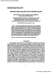
where m, v, e, B, and E are the mass, velocity, electric charge of electron, the magnetic field, and the electric field. The equation of motion is numerically solved by the Boris– Buneman version of the leap-frog method.4 Being based on the real magnet dimension and location 共see Fig. 1兲, the external magnetic field B at each local point is calculated in advance with the analytic solution based on the magnetic charge model.5 On the other hand, we assume the quasineutrality condition ne ⬇ ni 共ne: electron density, ni: ion density兲 in the bulk source region. The electric field E has not been taken into account in the present analysis, since the Debye length with a typical H− source plasma becomes relatively small except for the sheath layer at the plasma boundary. Various collision processes are taken into account in Eq. 共1兲 by Monte Carlo techniques. They are classified mainly
a兲
Contributed paper, published as part of the Proceedings of the 13th International Conference on Ion Sources, Gatlinburg, Tennessee, September 2009. b兲 Electronic mail:
[email protected]. 0034-6748/2010/81共2兲/02A703/3/$30.00
FIG. 1. 共Color online兲 The diagram of the JAEA 10 A negative ion source 共Ref. 8兲.
81, 02A703-1
© 2010 American Institute of Physics
02A703-2
Rev. Sci. Instrum. 81, 02A703 共2010兲
Terasaki et al.
TABLE I. Main reactions taken into account in the simulation.
TABLE III. Typical operation condition used in the simulation.
Collision species
Operation parameters
Reaction
eV EV H2 electronic excitation H electronic excitation H2 ionization H ionization
H2共v兲 + e → H2共v ⫾ 1兲 + e H2共X 1兺+g , v = 0.14兲 + e → H2共X 1兺+g , v⬙ = 0 , 14兲 + e e + H2共X 1兺+g 兲 → e + Hⴱ2共B1 兺+u 2p兲 e + H共1s兲 → e + Hⴱ共2p兲 e1 + H2共X 1兺+g 兲 → e1 + H+2 共v兲 + e2 e1 + H共1s兲 → e1 + H+ + e2
Dissociative attachment Recombination H2 elastic collision H elastic collision
e + H2共X 1兺+g ;v兲 → H− + H共1s兲 e + H+3 → 3H or H2共v ⬎ 5兲 + Hⴱ共n = 2兲 H2 + e → H2 + e H+e→H+e
into two categories. The first one is the collision processes of electrons with hydrogen particles 共H atoms, H2 molecules, H+, H+2 , and H+3 ions兲. Totally, about 540 collision processes are included in the analysis. Among these processes, main collision species are summarized in Table I. The second category is the electron-electron collision, i.e., Coulomb collision. The collision with hydrogen particles is modeled by the “null-collision 共NC兲” method6 to speed up the calculation, while the “binary collision 共BC兲” model7 is applied to Coulomb collision. The main procedure of NC method is summarized as follows. 共1兲 First, whether collision occurs or not is determined based on the maximum collision frequency. 共2兲 Next, when collision occurs, the kind of collisions is determined based on the ratio of collision frequency of each kind to the total collision frequency. The main procedure of BC method is summarized as follows. 共1兲 First, a pair of electrons is randomly chosen from the system and their relative velocity u is calculated. 共2兲 Next, the scattering angles, and ⌽, are calculated with the electrons density of the corresponding cell. The angle ⌽ is given by ⌽ = 2U, where U is a uniform random number. 共3兲 From these scattering angles, the relative velocity change ⊿u due to the collision is obtained. 共4兲 Finally, the velocity change in each electron involved in the collision is calculated. III. NUMERICAL SIMULATION OF JAEA 10A SOURCE
We applied our simulation code described in Sec. II to the analysis of the EEDF in JAEA 10A source.8 Figure 1 shows the diagram of the source. In the simulation, the realistic source dimension, geometry, magnetic configuration, and filament locations are taken into account. We adopted the 共X , Y , Z兲 coordinate system shown in Fig. 1. The model dimensions are summarized in Table II. In the experiments, 66 magnets are installed surrounding the vacuum chamber, as schematically shown in Fig. 1. The number, dimension, and
Parameters’ values
Arc power Arc voltage Arc current Pressure
10 kW 60 V 166.6 A 0.3 Pa
location of these cusp and filter magnets in our simulation are exactly the same those in the experiments. The resultant magnetic field inside the source is calculated by the surface magnetic charge model5 as mentioned above. Being based on a typical operation condition of the JAEA 10A source, the operational parameters in our simulation are calculated and summarized in Table III. The initial energy of the primary electrons emitted from the filaments is set to be 60 eV with the assumption that these electrons are accelerated by the arc voltage in the thin sheath region surrounding the filaments immediately after their thermal emission. The emitted angle is chosen from the isotropic distribution for simplicity. The number of electron test particles emitted from the filaments at each time step and the statistical weight of each test electron are determined from the arcdischarge current in Table III. With above initial conditions, trajectories of test electros are followed by Eq. 共1兲 with the numerical time step ⌬t = 10−10 s, which is much smaller than the Larmor period in the magnetic field inside the source. The time step ⌬tNC and ⌬tBC for the NC method and the BC model are chosen, respectively, as ⌬tNC = 10−8 s and ⌬tNC = 10−8 s. The former is much smaller than the minimum flight time of the NC method and the latter is chosen so as to simulate the important feature of the small angle scattering of the Coulomb collision. The main collision processes included in the simulation has already been shown in Table I. The main simulation parameters related to the collision processes with hydrogen particles, which are necessary to calculate the collision frequency used in the NC method, are summarized in Table IV. In order to take into account the sheath-potential drop near the walls and PG, here, we used the following simple model. If these test electrons reach the upper/side/bottom walls, those electrons with the energy Ee larger than the sheath-potential drop 共Ee ⬎ e兩Vsh兩, where Vsh is the sheathpotential drop兲 are absorbed at the wall, while those with the low energy 共Ee ⱕ e兩Vsh兩兲 are reflected. The sheath-potential drop Vsh can be estimated from the sheath theory,9 Vsh ⬇ 共kTe / 2e兲ln关共1 / 2兲共mi / me兲兴, where Te and mi are the elecTABLE IV. Parameters for the hydrogen species. Simulation parameters
Parameter values
TABLE II. Dimensions of the sources in our model.
Direction of the axes in the source Transversal direction 共X兲 Longitudinal direction 共Y兲 Extracting direction 共Z兲
Length 共mm兲 −120⬍ X ⬍ 120 −240⬍ Y ⬍ 240 0 ⬍ Z ⬍ 203
Hydrogen Hydrogen Hydrogen Hydrogen Hydrogen Hydrogen Hydrogen
molecule temperature TH2 molecule density nH2 atom temperature TH atom density nH ion density nH+ ion density nH+ 2 ion density nH+ 3
300 K 共initial兲, 2000 K 共during discharge兲 2.8⫻ 1019 m3 5802 K 2.8⫻ 1018 m3 H+ : 4 ⫻ 1017 H+2 : 1.0⫻ 1017 H+3 : 5.0⫻ 1017
02A703-3
Rev. Sci. Instrum. 81, 02A703 共2010兲
Terasaki et al.
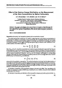
FIG. 4. 共Color online兲 The EEDF in the driver region and the extraction region. FIG. 2. 共Color online兲 Magnetic configuration in 共X, Z兲 cross section 共at Y = 0兲. The “driver” region and “extraction” region are, respectively, defined by shaded regions in the figure.
tron temperature and ion mass, respectively. In the present simulation, 兩Vsh兩 = 14 V and 兩Vsh兩 = 3 V are assumed, respectively, for the top/side/bottom walls and the PG 共plasma grid兲 with typical electron temperatures in the experiments 共Te ⬇ 3 eV in the driver region, Te ⬇ 1 eV while near the PG兲. We also parametrically changed Vsh in the range 兩Vsh兩 = 3 – 15 V. The results, however, do not depend so much on the assumption for the 兩Vsh兩 at least in the present simulation. In order to discuss the spatial variation of the EEDF, we divide the discharge volume into two typical regions in the 共X , Z兲 cross section of the discharge chamber and defined as the “driver” region and “extraction” region, as shown in Fig. 2 IV. RESULTS AND DISCUSSION
Figure 3 shows the EEDF of the driver region in Fig. 2, more precisely, the value of EEDF/ E1/2 共EEDF divided by 冑E兲, is plotted in the log scale. The EEDF at the top 共Y = +220 mm兲 in the longitudinal 共Y兲 direction in Fig. 2 is compared with that at the bottom 共Y = −220兲. The high energy electrons exist at the top of the ion source rather than at the bottom. This nonuniformity of the EEDF, caused by B ⫻ ⵜB drift, is also observed in experiment.1 Also, it should be noted that the calculated EEDF consists of mainly two energy groups: 共1兲 low energy group
共⬍20 eV兲 and 共2兲 high energy group 共⬎20 eV兲. The temperature of each energy group can be estimated from the slope of the EEDF/ E1/2 in Fig. 3. The results become Te ⬃ 3 eV for the low energy group, while Te ⬃ 20 eV for the high energy group. These results are in good agreement with the experimental results Te ⬃ 3 – 5 eV and Te ⬃ 20 eV,1 by the two-temperature fit of the Langmuir probe data. Coulomb collision seems to play a key role for the low energy part, while in elastic collision for the high energy range 共E ⬎ 30 eV兲. Next, we fix the longitudinal position 共Y = 0兲, which is the center position of the discharge chamber, and make a comparison of the EEDF for the “driver” and “extraction” region in Fig. 2. As seen from Fig. 4, the number of high energy electrons 共⬎20 eV兲 is effectively reduced in the extraction region due to the magnetic filter effect on the high energy electrons. A spatial nonuniformity of plasma density on a plasma grid is not reproduced in this study. We observed only a spatial nonuniformity of driver region. We presume the nonuniformity on a plasma grid from the result. Now, we are improving the code to reproduce the nonuniformity. Although further validation and improvements of the model are required, the above results show that the developed 3D simulation code of the EEDF is a useful tool not only to understand the basic physics, but also to design the new H− ion sources. 1
FIG. 3. 共Color online兲 Comparison of the EEDF in the driver region: at the top 共Y = +220兲 and at the bottom 共Y = −220 mm兲.
N. Takado, H. Tobari, T. Inoue, J. Hanatani, A. Hatayama, M. Hanada, M. Kashiwagi, and K. Sakamoto, J. Appl. Phys. 103, 053302 共2008兲. 2 C. Gorse, M. Capitelli, M. Bacal, J. Bbetagne, and A. Lagana, Chem. Phys. 117, 177 共1987兲. 3 I. Fujino, A. Hatayama, N. Takado, and T. Inoue, Rev. Sci. Instrum. 79, 02A510 共2008兲. 4 C. K. Birdsal and A. B. Langdon, Plasma Physics via Computer Simulation 共McGraw-Hill, New York, 1985兲, pp. 13–15 and 58–63. 5 Y. Ohara, M. Akiba, H. Horiike, H. Inami, Y. Okumura, and S. Tanaka, J. Appl. Phys. 61, 1323 共1987兲. 6 K. Nanbu, IEEE Trans. Plasma Sci. 28, 971 共2000兲. 7 T. Takizuka and H. Abe, J. Comput. Phys. 25, 205 共1977兲. 8 M. Hanada, T. Seki, N. Takado, T. Inoue, H. Tobari, T. Mizuno, A. Hatayama, M. Dairaku, M. Kashiwagi, K. Sakamoto, M. Taniguchi, and K. Watanabe, Rev. Sci. Instrum. 77, 03A515 共2006兲. 9 G. A. Emmert, Phys. Fluids 23, 803 共1980兲.