3D Modeling Visualization for Studying Controls of the Jumbo. Container Crane. J.B. Klaassens, G. Honderd, A. El Azzouzi,. Ka C. Cheok. , G.E. Smid.
American Control Conference, San Diego June 1999, pp. 1754-1758
3D Modeling Visualization for Studying Controls of the Jumbo Container Crane J.B. Klaassens, G. Honderd, A. El Azzouzi, Ka C. Cheok�, G.E. Smid�, Faculty of Information Technology and Systems Control Laboratory Delft University of Technology
Backreach
Span
Outreach
Abstract The jumbo container cranes at the European Container Terminal (ECT) in Rotterdam are subject of a long term study to automate the international seaport and make container handling more efficient. In this paper appropriate details of the 3D dynamical behavior of the container is modeled. Simulation and visualization are carried out to study the crane behavior under disturbing conditions like unbalanced center of gravity and varying side winds. The software is used to evaluate time-optimal trajectories and control schemes for the dynamics of the electrical drives, and of the swing and skew of the container.
8000 TEU-ship
L2
L1 Quay
Figure 1: A schematical drawing representing loading and Keywords : Container crane, 3D dynamics model, swing unloading of the Jumbo Container Crane. and skew control, gantry crane.
1 Introduction
construction of the crane, the stretch in the cables and the influence of wind. A six degree of freedom (dof) model is presented in this paper to study the other modes like skew and sway. These modes will be excited by the unsymmetric characteristics of hoisting ropes, unbalanced loading of the container and the influence of wind. This model allows control schemes for the dynamical movements of the container to be studied extensively. A control concept that introduces a time-optimal trajectory [4] while minimizing the swing and the wind influence, is presented. The structure of the paper is as follows. Section 2 presents the basic equations to obain the 3D model of the container crane. Section 3 presents the control scheme and Section 4 shows the simulation results of the dynamic behavior of the crane.
The need for fast and safe loading and unloading container vessels whose service time is to be minimized, requires a control of the crane motion that optimizes the crane’s dynamic performance. The two-dimensional cycle is divided in three motions: load hoisting, transfer and load lowering. The problems are the reduction of the total time of load transport (time-optimal trajectory control [1], [4]) and reduction of the swing of the load at its end position, including accurate positioning of the load. During the transport of the load, the planar position is controlled by varying the position of the trolley and varying the length of the suspension rope. Specific constraints such as maximum torque (which is a maximum acceleration or deceleration of the trolley or load), maximum speed and the existance of obstacles on the quay or in the container vessel, have to be incorporated in the trajectory controller. 2 Modeling A validated math model is necessary for conducting detailed study of the dynamic behavior of the container crane and control schemes. Although several analyses have been Figure 1 shows a drawing of the side elevation of the crane made, using nonlinear models [5], [6], further increased that is being studied in this paper. In order to model the complexity may be considered by including the detailed motion dynamics of the container body, we assign two coordinate reference frames. They are the global reference � Department of Electrical and Systems Engineering, Oakland Uni- frame, on the base of the rail, and the container attached reference frame, in the geometric center of the container. The versity, Rochester MI, USA.
A1
The forces in the cables are given by
A2
� o� � F�i = jDDij Ks Si + Kd S_i
A4 A3
A1
o
xT
A2
where Ks is the stiffness and Kd the damping coefficient, and Si is the stretch, computed as
C2
C1 C4
Si = jDi j , Li :
C3
C1
(8)
i
C2 z
(9)
Here, Li is the unloaded length of cable i. The total force acting on the container and the spreader is the sum of cable forces oFi, together with the wind force o W and the gravo itational force G, where is the mass matrix. The acceleration vector of the C.G. of the container thus becomes !
c.g.
�
y x
M �
�
M
X �a = M ,1 oW� + oF�i +o G:�
Figure 2: Geometry of trolley, container and cables.
o
(10)
i
following notation will be adopted throughout this paper
Since velocity and position can be found by integration of acceleration, the dynamic equations for the container mass ; (1) can be represented in the diagram in Figure 3, where is a matrix or vector. A vector with respect to the global reference frame will be denoted with o , and Σ F+ W a v x 1 1 M-1 with respect to the container reference frame with c . Fur+ s s thermore, matrices will be printed in bold, and vectors with overbar. 0 The transformation from the global reference frame to the G o container frame is defined by C , [2] as frame
V
V
V V
R RC = RxRy Rz
o
where
cos( ) sin( ) 0 # Rz = , sin( ) cos( ) 0 0 0 1 " cos(�) 0 sin(�) # 0 1 0 Ry = , sin(�) 0 cos(�) " 1 0 0 # Rx = 0 cos(�) sin(�) : 0 , sin(�) cos(�) "
o
o
0
i
0
0
(2) Figure 3: Model for container translational motion dynamics A state space model description for the translational container motion can be expressed as (3) d dt
(4)
�
o o
� �
�� = 0 0 x� I 0
��
o o
� �
�� + M ,1 (P o F i +o W )+ G x� 0
�
(11)
The sum of the torques acting on the container and spreader can be computed by (5)
o
4
X, oC �i ,o x�� � oF�i + ox�w � oW: � T� = i=1
(12)
where �, � and are the Euler angles representing roll, pitch and yaw of the container. where � denoted a cross-product operation. Taking the centrifugal and coriolis acceleration into account, the instantaneous angular accelerations with reference to the container 2.1 Container Dynamics frame can be derived as Figure 2 shows the configuration of the trolley and container � , �� c system. It is clear from Figure 2, that the displacement I ,1 o TC o T , c � I �c : (13) vectors for the cables can be stated as
�_ = �
R �
� ( � � ) � can be found by inThe container gyroscopic angle rate c
tegration. In order to find the rotation angles of the container, c
� needs to be translated to Euler angle rates o��_ . With ~i,
D� i =o A�i ,o C�i for i = 1 : : : 4 (6) o The locations of the pulleys A�i on the trolley can be derived from the trolley position on the rail xT and the geometric ~ �i on the j and ~k being the unit vectors in the x, y and z-directions design of the crane. The locations of the pulleys o C respectively, the transformation o
container are derived from the motion of the container: o
C�i = x� + o RC c C�i
(7)
Rf = Rz Ry Rx~i + Rz Ry~j + Rz~k
(14)
provides the relation o
then the drive control system can be represented in state space form as
��_ = Rf c � :
(15)
The body rotation angles �, � and can be found by integration of the above equation, as the elements of o . The diagram in Figure 4 represents the model for the angular dynamics.
��
Σ ( C - x)× F 4
o
o
o
i
i
i=1
+ o
R
c
T C
T
-1
I
-
c
Ω
1 s
c
Ω
Rf s
c
Ω × ( cΩ • I )
c
The coriolis and centrifugal torques can be expressed in a matrix product as follows
SI � =c � � I � � c
where
S is given by
"
0
,!z !y # S = !z 0 ,!x : ,!y !x 0
Ui Ia ! x
7 5
=
6 6 6 6 6 6 6 4 2 6 6 6 6 6 6 4
0 ,Ki 0 1 ,Kp + R , Kb L L L KT Fv 0 J J 1 0 03 N KI 0 KP 0 777 � � 7 I ref L 7 �load 1 0 J 75 0 0
0 0 0 0
3 72 7 7 76 74 7 7 5
Ui Ia ! x
3 7 5
(20)
In this formulation, Ui stands for the control output of the integral part of the PI-current controller and Iref is the reference current command. The load torque �load on the hoist drive shaft, caused by the force in the cables, is modeled as
Figure 4: Model for the angular dynamics
c �
d 6 dt 4
3
+
θ
xw×oW
,
2 2
(16)
�load = dN�
X i
o
F�i:
(21)
Trolley drive. The control and dynamics model for the hoisting drive system does also apply to the DC machine that drives the trolley system. However, the feedback load torque for the trolley system is the horizontal component of (17) the forces in the cables,
The state space formulation for the angular dynamics is given by:
�load = dN� sin(�)
X i
o
F�i
(22)
where � is the swing angle. Skew drive. The skew drive system consists of a motor actuation that can shift one side (two cables) of the hoist mechanism on the trolley forward and backward so that the cables apply a yaw torque on the container and and spreader. 2.2 Hoist, Trolley and Skew Drives Again, the similar model of the DC-drive and motor system Hoist Drive. The hoisting system is configured with four can be applied to describe the skew control drive. 350 kW DC motors that are mechanically connected to the drum shaft through a gear box. The gearbox is configured 2.3 State Space Formulation to optimize the power-speed ratio of the system. In order to control the force in the hoisting cables the The objective for the space container crane system modeling armature currents of the motors are controlled. This requires is to derive a parameterized input-output formulation, that an extra feedback of the motor currents. The drive system will predict motions and forces of the container and the model is graphically represented in the diagram in Figure 5. trolley, for a given trajectory R and a given set of electric drive controllers CT , CH and CS (The controller design schemes will be discussed in the following section). τ ω = DC Motor shaft spin velocity x = Drum angular position From this perspective, Equations (6), (8) and (12) can be I I U used to express the inputs of the systems (11), (18) and (20) ω x 1 + 1 1 K C - Ls+R Ns Js+F as functions of each others states. Only for the input currents to the DC drives we need the expression for the controller models as functions of the system states. K As shown in Figure 6, the control strategy consists of a trajectory planner and a set of controllers (CT , CH and Figure 5: A typical linear model for the DC Drive and Motor CS ) for controlling the motion of the container. In this systems paper we will present only some examples of the simple controllers that have been used to illustrate the simulation When a PI-controller is considered for the current con- and visualization aspects of the crane project. We remarked the several extensive studies such as time troller , optimal control [4], model predictive control [3], etc, that s KP KI s ; (19) have been conducted and will be reported in the future. d dt
� � = � ,I ,1SI 0 � � c � � + � I ,1RC � oT
o� � Rf 0 o �� 0
�c
load
ref
a
T
v
b
C
C( ) =
+ 1
(18)
Setpoints and Environmental Conditions
rT
Time Optimal Trajectory Planner
Swing Controller CT
Current Command Iref,swing
xT Trolley vT System Dynamics
Trolley and Hoist Cables
o o
rH
rS
Hoist Controller CH
Skew Controller CS
Current Command Iref,hoist
Iref,skew
xH Hoist vH System Dynamics
Container and Spreader Dynamics
F T
o
x v o θ o θ o
xS Skew vS Control Mechanics
Figure 6: Overview of the control strategy for the Container Crane System.
3
Control
An important objective of the automated container crane system is to regulate the swing motion of the container. The criterion for controller design for transfering a container from the ship to the shore concerns with the time of travel that begins when the spreader locks onto a container and which ends as soon as the container hangs just above its end location with an error of less than 5 cm. For this purpose a time-optimal trajectory is planned (details can be found in [4]) and used as a reference path for the container to follow. The control strategy therefore is to “drive” the container along the time-optimal path in the quickest manner while minimizing the swing and skew in the motion.
3.1
Swing Control
equal in length. Once the swing period for the left and right side of the container will be different. Additionally, skew can be caused by side wind as well as unbalanced loading in the container. Several methods exist for controlling skew motion. The two methods of interest are
� �
xC = xT + L^ i + 12 hC sin(�) �
Shifting of the left or right pulley’s along the xdirection of the trolley, which will effectively apply an additional skew torque as damping on the disturbance skew motion.
The latter method is used in the simulation described in this paper. The pulley positions on the trolley on the left rail are given by
The horizontal container position can be expressed as �
Independent control of the left and right hoisting cable lengths, which will effectively change the swing time of the left and right hoisting cables;
�
A�i (x) = A�i+2 (x) + �S
for i
= 1; 2
(25)
where S represents the pulley positions difference between (23) the left and the right side of the trolley. For our illustration, the skew controller is implemented as a damper, i.e.
:
=
_
which is the trolley position plus the offset of the container CS Iref;skew KS : (26) caused by swing. hC denotes the height of the container and Li is the actual length of the cables when they are stretched. where is the skew rate. In the control scheme, xC is subtracted from the reference input for container position xR . Furthermore, the trolley 3.3 Hoist Control speed xT , swing angle � and swing velocity � are fed back. Similarly, the hoist control is implemented as a P-controller, The swing dynamics are sensed with a CCD camera. For our illustration, the swing controller CT is defined by CH Iref;hoist KH Lref , Li : (27) CT Iref;swing KT;swing xref;T (24)
_
^
_
_
:
=
:
[
, xC , KT;x_ x_ T + KT;� � , KT;�_ �_ ]
4
=
(
^)
Simulation & Animation
Figure 7 shows the signals for trolley position, container position and swing angle in a simulation of the container Skew is the name for the angular motion about the vertical for moving from the center to the left and to the far right in axis of the container. It is measured using two CCD cameras. the work plane. Also a 3D animation of the crane has been It occurs when, for example, the left and right cables are not developed.
3.2
Skew Control
[6] Y. Sakawa and Y. Shindo. Optimal control of container cranes. Automatica, 18(3):257–266, 1982. -XPER�&UDQH�6LPXODWLRQ�5HVXOWV
[7] D.T. Greenwood. Principles of Dynamics, Prentice Hall, Englewood Cliffs, NJ, 1965.
50.00 40.00 30.00 20.00 10.00
-20.00
7UROOH\�;
-30.00
6ZLQJ�DQJOH
59.40
53.40
47.40
41.40
35.40
29.40
23.40
17.40
11.40
5.40
Tijd
0.00 -10.00
6NHZ�$QJOH
-40.00
&DEOH�/HQJWK -50.00
5HI�;
-60.00
7LPH��V
[8] G.E. Smid, Ka C. Cheok and T.K. Tan, Multi-CPU real-time simulation of vehicle systems. Proceedings of the 7th International Conference on Intelligens Systems (ICIS ’98) Melun Fontainebleau, France July 1-2 1998. [9] G.E. Smid, Ka C. Cheok and K. Kobayashi, Modeling of Vehicle Dynamics using Matrix-Vector Oriented calculations in Matlab. Proceedings of the ISCA 9th International Conference on Computer Applications in Industry and Engineering (CAINE), Orlando, FL, Dec 11-13, 1996.
Figure 7: Simulation output results of trolley and container [10] K. Kobayashi, K. Watanabe, Ka C. Cheok and G.E. Smid, S Simple Vehicle Dynamics Modeling usig position xT and swing angle � as a function of time. Object Oriented Approach. Japan Journal of Instrumentation and Control Engineering, Jan 7, 1997.
5
Conclusions
[11] C. Burhenne, G. Honderd and J.B. Klaassens, Modeling the non-linearities and non-stiffness of a Jumbo The 3-D math model for the dynamics of hoisting a conContainer Crane. Technical report, Control Lab, Factainer with the JCC 2000 Jumbo Container Crane has been ulty of Information Technology and Systems, Delft Unipresented. The drives and the control schemes have been versity of Technology. Delft, the Netherlands, June 29, discussed. 1998. Simulation results with a simple controller to stabilize the swing and the skew of the container have shown satisfying and promising results. The modeling and the controller design for the Jumbo Container Crane is a big and involved task. For example, the time-optimal control must not only move the container quickly to its destination, but also do this within the numerous constraints for currents torques and speeds, but also within a positioning accuracy of 5 cm. Other more sophisticated control solutions will follow in future papers.
References [1] J. W. Auernig and H. Troger. Time optimal control of overhead cranes with hoisting of the load. Automatica, 23(4):437–447, 1987. [2] A. Craig. Introduction to Robotics. Addison Wesley, 3rd edition, 1996. [3] Peter J. Van der Veen. Trajectregelaar voor containerkranen (i). Master’s thesis, Delft University of Technology, 1998. [4] P. Hippe. Time optimal control of an overhead crane. Regeltechnik und Prozess-Daten arbeitung, 18(8):346– 350, 1970. [5] A. J. Ridout. Anti swing control of the overhead crane using linear feedback. Journal of Electrical and Electronic Engineering, pages 17–26, 1989.