SS symmetry Article
3D Reconstruction Framework for Multiple Remote Robots on Cloud System Phuong Minh Chu 1 , Seoungjae Cho 1 , Simon Fong 2 , Yong Woon Park 3 and Kyungeun Cho 1, * 1 2 3
*
Department of Multimedia Engineering, Dongguk University-Seoul, 30, Pildongro-1-gil, Jung-gu, Seoul 04620, Korea;
[email protected] (P.M.C.);
[email protected] (S.C.) Department of Computer and Information Science, University of Macau, Avenida da Universidade, Taipa, Macau SAR 3000, China;
[email protected] Institute of Defense Advanced Technology Research, Agency for Defense Development, P.O. Box 35, Yuseong, Daejeon 34186, Korea;
[email protected] Correspondence:
[email protected]; Tel.: +82-2-2260-3834
Academic Editors: Doo-Soon Park and Shu-Ching Chen Received: 13 December 2016; Accepted: 7 April 2017; Published: 14 April 2017
Abstract: This paper proposes a cloud-based framework that optimizes the three-dimensional (3D) reconstruction of multiple types of sensor data captured from multiple remote robots. A working environment using multiple remote robots requires massive amounts of data processing in real-time, which cannot be achieved using a single computer. In the proposed framework, reconstruction is carried out in cloud-based servers via distributed data processing. Consequently, users do not need to consider computing resources even when utilizing multiple remote robots. The sensors’ bulk data are transferred to a master server that divides the data and allocates the processing to a set of slave servers. Thus, the segmentation and reconstruction tasks are implemented in the slave servers. The reconstructed 3D space is created by fusing all the results in a visualization server, and the results are saved in a database that users can access and visualize in real-time. The results of the experiments conducted verify that the proposed system is capable of providing real-time 3D scenes of the surroundings of remote robots. Keywords: 3D reconstruction; ground segmentation; cloud system; point cloud
1. Introduction Nowadays, various innovative technological systems, such as multimedia contexts [1–6], video codecs [7,8], healthcare systems [9,10], and smart indoor security systems [11,12] are being actively researched. In the area of cloud computing, a failure rules aware node resource provision policy for heterogeneous services consolidated in cloud computing infrastructure has been proposed [10]. Various applications for human pose estimation, tracking, and recognition using red-green-blue (RGB) cameras and depth cameras have also been proposed [13–24]. A depth camera gives an image in each frame that contains information about the distance from the camera to other objects around the camera’s position. In contrast, an RGB camera gives a color image in each frame. The security problems in distributed environment and cloud database as a service (DBaaS) have also been studied [25–27]. Cloud computing [28,29] provides shared computer processing resources and data to computers and other devices on demand. In this study, we employed the cloud model to create a three-dimensional (3D) reconstruction framework for multiple remote robots. The 3D reconstruction [30–36] has been widely studied as an approach to enhance the sense of reality and immersion for users. However, accomplishing this technique in real-time and with high quality is challenging, particularly with multiple remote robots. In many tasks, such as rescue or tracking terrain, multiple remote robots are required to expand the working area. Each robot often has a light detection and ranging (Lidar) Symmetry 2017, 9, 55; doi:10.3390/sym9040055
www.mdpi.com/journal/symmetry
Symmetry 2017, 9, 55
2 of 16
sensor, several cameras, and an inertial measurement unit-global positioning system (IMU-GPS) sensor attached. A Lidar sensor returns a point cloud that senses the surface of the terrain around the robot. The cameras are either 2D or stereo, and the images obtained from them are used to compute color points or texture coordinates. The IMU-GPS sensor is used to check the position and direction of each robot. An enormous amount of data is obtained from the multiple sensors attached to each robot. Processing these bulk data in real-time is impossible using a single computer with limited power. Thus, we propose a cloud system that optimizes the reconstruction of these large amounts of sensor data from multiple remote robots. In this framework, we create a master-slave server model in which the master server distributes the data to be processed to multiple slave servers to increase the computing ability. The segmentation servers use our previously proposed algorithm [37] to separate each frame of the point cloud data into two groups: ground and non-ground. The first group consists of ground points of terrain that the robots can traverse. The second group consists of non-ground points that the robots cannot traverse, such as buildings, walls, cars, and trees. The reconstruction servers process the ground and non-ground data differently. Furthermore, the non-ground data are modeled using colored particles [35]. On the other hand, the ground data are reconstructed by meshing and texture mapping [36]. The results from all reconstruction servers are then sent to a visualization server to save in a database. We employ a file database where users can access and visualize the 3D scene around all the robots. 2. Related Works Reconstruction of 3D scenes from point clouds is an important task for many systems such as autonomous vehicles and rescue robots. Several studies have been conducted on reconstruction in both indoor and outdoor environments [30–36]. In the indoor environment, Izadi et al. [30] and Popescu and Lungu [31] employed a Microsoft Kinect sensor. Khatamian and Arabnia [32] reviewed several 3D surface reconstruction methods from unoriented input point clouds and concluded that none of them are able to run in real-time. In [33–36], the authors used one 3D laser range scanner combined with cameras and an IMU-GPS sensor for the outdoor environment. Because the features of ground and non-ground data are different, they have to be segmented and reconstructed separately. Over the past few years, many segmentation methods [38–43] have been proposed. However, these methods have disadvantages related to accuracy and processing time. We previously introduced a new ground segmentation algorithm [37] that works well with various terrains at high speed. Paquette et al. [44] employed orthorgonal lines to determine the orientation of the mobile robot. In [45,46], the authors proposed a method for navigating a multi-robot system through an environment while obeying spatial constraints. Mohanarajah et al. [47] presented architecture, protocol, and parallel algorithms for collaborative 3D mapping in the cloud with low-cost robots. Jessup et al. [48] proposed a solution for refining transformation estimates between the reference frames of two maps using registration techniques with commonly mapped portions of the environment. Another study [49] investigated a visual simultaneous localization and mapping (SLAM) system based on a distributed framework for optimization and storage of bulk sensing data in the cloud. In [50,51], the authors supplemented the insufficient computing performance of a robot client using a cloud server for collaboration and knowledge sharing between robots. Sim et al. [52] proposed a calibration scheme for fusing 2D images and 3D points. For fast transfer data among the computers in the network, we use the UDP-based data transfer protocol (UDT) [53] which UDP stands for user datagram protocol. This method can transfer data at high speeds (10 Gbit/s). In our research, the data are compressed to decrease the bandwidth for transmission via the network and reduce storage space in the database. The compression is an important task in many studies [54–57]. There are two types of compression: lossy and lossless. For 2D images, we use a lossy compression method, and a lossless compression method is employed for other data. We employ a fast and high ratio compression method library [58]. The studies cited above involve server-based data processing technology for processing bulk sensor data generated from a number of clients. The insufficient computing performance of the client
Symmetry 2017, 9, 55
3 of 16
Symmetry 2017, 9, 55
3 of 16
was obviated by employing a distributed processing environment using a cloud server. However, The studies cited above involve server-based data processing technology for processing bulk one common feature of the studies cited above is reliance on batch-processing methods, rather than sensor data generated from a number of clients. The insufficient computing performance of the client real-time processing. contrast,a we proposeprocessing a real-time platformusing for the reconstruction of 3D scenes was obviated byIn employing distributed environment a cloud server. However, from point clouds and 2Dofimages acquired by sensors attached to multiple methods, robots. rather than one common feature the studies cited above is reliance on batch-processing real-time processing. In contrast, we propose a real-time platform for the reconstruction of 3D scenes
3. Framework Design from point clouds and 2D images acquired by sensors attached to multiple robots. The 3D reconstruction framework acquires data from multiple sensors attached to 3. cloud-based Framework Design multiple remote robots. The data are used to reconstruct the 3D scene in real-time. Figure 1 gives an The cloud-based 3D reconstruction framework acquires data from multiple sensors attached to overview of theremote framework. Suppose have n remote robots workingFigure simultaneously, each multiple robots. The data are that used we to reconstruct the 3D scene in real-time. 1 gives an with k sensors several 2D cameras, 3D nrange sensor, an IMU-GPS. The 2D overviewcomprising of the framework. Suppose that we ahave remote robotsand working simultaneously, eachcameras with kimages sensors of comprising several 2Daround cameras,each a 3D robot. range sensor, and an IMU-GPS. 2D cameras return color the environment In each frame, the 3DThe range sensor releases return color images of the environment around each robot. In each frame, the 3D range numerous laser rays and returns a point cloud. The IMU-GPS sensor is used to detectsensor the position releases numerous laser rays and returns a point cloud. The IMU-GPS sensor is used to detect the and navigation of each robot. We therefore construct a framework that creates a working environment position and navigation of each robot. We therefore construct a framework that creates a working for these n robots in real-time. The framework contains one master server, one visualization server, environment for these n robots in real-time. The framework contains one master server, one m segmentation servers, and m reconstruction servers (m ≥ n). Each hasEach onerobot computer that visualization server, m segmentation servers, and m reconstruction serversrobot (m ≥ n). has acquires allcomputer the datathat from multiple sensors. Themultiple data are compressed sending to the master one acquires all the data from sensors. The databefore are compressed before sending to thecommunication. master server via wireless communication. server via wireless
Figure 1. Overview of our three-dimensional (3D) reconstruction framework based on the cloud for Figure 1. Overview of our three-dimensional (3D) reconstruction framework based on the cloud for multiple remote robots. multiple remote robots.
After considering the computing resources of all slaves, the master distributes the data to the m segmentation servers. each segmentation server, are decompressed, then, by using After considering theIncomputing resources of the all data slaves, the master distributes theIMUdata to the GPS data, and all points are converted from local to global coordinates. We separate the point cloud m segmentation servers. In each segmentation server, the data are decompressed, then, by using into two parts: ground and non-ground. The segmentation result is again compressed before being IMU-GPS data, and all points are converted from local to global coordinates. We separate the point sent to its corresponding reconstruction server. In each reconstruction server, all of the data are first cloud into two parts: ground and non-ground. The segmentation result is again compressed before decompressed and then used to reconstruct the virtual 3D scene. Then, the results from all being sent to its corresponding reconstruction server. In each reconstruction server, of the data reconstruction servers are compressed again and transferred to the visualization server to beall saved are firstindecompressed and then reconstruct virtual 3Dscene scene. Then, thearea results the database. Users can thenused accessto the database andthe obtain the 3D of the working of allfrom all the remote robots.are compressed again and transferred to the visualization server to be saved in reconstruction servers the database. Users can then access the database and obtain the 3D scene of the working area of all the 3.1. Ground Segmentation Algorithm remote robots. We employ our ground segmentation algorithm [37]. The main idea of this algorithm is to divide a point cloud into small groups, each called a vertical-line. The pseudo-code representing our idea is 3.1. Ground Segmentation Algorithm shown in Algorithm 1. First, we decompress the point cloud and IMU-GPS data. As the frame data
Wegained employ ourtheground segmentation [37]. The of thisthem algorithm is to divide from range sensor are in thealgorithm local coordinates, wemain have idea to convert into global employ the method presented in [35] to change coordinates ofrepresenting all 3D points inour idea a point coordinates. cloud into We small groups, each called a vertical-line. Thethe pseudo-code each dataset with small we distortions. For example, robot cloud #k startsand collecting 3D points at time . frame is shown inframe Algorithm 1. First, decompress the point IMU-GPS data. As the At time , the local coordinate system of a 3D point is centered at robot position . To change data gained from the range sensor are in the local coordinates, we have to convert them into global the coordinate system of all points, we use the following formula: coordinates. We employ the method presented in [35] to change the coordinates of all 3D points in each frame dataset with small distortions. For example, robot #k starts collecting 3D points at time ti . At time tj , the local coordinate system of a 3D point PC is centered at robot position Lj . To change the coordinate system of all points, we use the following formula: PG = Rj ( PC + L0 ) + Lj − Li
(1)
Symmetry 2017, 9, 55
4 of 16
Symmetry 2017, 9, 55
4 of 16
where L0 is the 3D vector from the 3D sensor location to the GPS sensor location. Li is the 3D vector from the starting position of robot #k to one fixed point, which is chosen as an origin of the global (1) coordinate. Rj is the rotation matrix of robot #k at time tj . The error of this method is only a few where Inisaddition, the 3D vector the 3D location to the GPS sensor location. is the vector centimeters. thisfrom method issensor capable of merging point clouds captured by3D many robots. the startingwe position of robot #k toand one non-ground fixed point, which is separately chosen as an originsending of the global After from segmentation, compress ground groups before them to a coordinate. is the rotation matrix of robot #k at time . The error of this method is only a few corresponding reconstruction server. centimeters. In addition, this method is capable of merging point clouds captured by many robots. After segmentation, we compress ground and non-ground groups separately before sending them to Algorithm 1 Ground segmentation a corresponding reconstruction server. Convert all points into global coordinate() FOR EACH vertical-line IN segmentation a frame data Algorithm 1 Ground WHILE NOT (all points the vertical-line Convert all points intoin global coordinate()are labeled) Assign a start-ground point() FOR EACH vertical-line IN a frame data Find a threshold point() WHILE NOT (all points in the vertical-line are labeled) Assign points’ label() Assign a start-ground point() END Find a threshold point() END Assign points’ label() END END
3.2. Terrain Reconstruction Algorithm
3.2. Terrain Reconstruction Algorithm the 3D terrain is based on the ideas presented in [35,36]. The method used to reconstruct The architecture running reconstruction serverisisbased illustrated Figure 2. Following theThe ground The method usedintoeach reconstruct the 3D terrain on the in ideas presented in [35,36]. segmentation step, each set of frame data is divided into two groups. We apply a projection method architecture running in each reconstruction server is illustrated in Figure 2. Following the ground usingsegmentation texture buffers non-ground A set ofinto colored points We is obtained using themethod calibration step,and each set of frame points. data is divided two groups. apply a projection using texture buffers andpoints non-ground points. set of colored obtained the calibration method [52]. These colored are split intoAseveral nodespoints basedison the x–zusing coordinates. Then, the method result [52]. These colored points are split intoand several on the x–zserver. coordinates. Then, the non-ground of each node is compressed sentnodes to thebased visualization The ground points non-ground result of each node is compressed and sent to the visualization server. The ground points are used to update the ground mesh, which is a set of nodes. The size of each ground node is equal to areof used update the ground mesh, which is aWe setthen of nodes. The size of eachmapping ground node equal the size theto non-ground node outlined above. implement texture fromisthe ground to the size of the non-ground node outlined above. We then implement texture mapping from the mesh and texture buffers. The ground surface result is also compressed and sent to the visualization ground mesh and texture buffers. The ground surface result is also compressed and sent to the server. We employ the zip library (ZLIB) [58] for compression and decompression because it is lossless visualization server. We employ the zip library (ZLIB) [58] for compression and decompression and fast. Each inand Figure is described in detail in [35,36]. However, sending the sending ground and because it isblock lossless fast. 2Each block in Figure 2 is described in detail in [35,36]. However, non-ground reconstruction result data is a challenging even after compressing the data. More the ground and non-ground reconstruction result data istask, a challenging task, even after compressing details the sending result data are given the are ensuing section. theofdata. More details of the sending resultindata given in the ensuing section.
Figure 2. Terrain reconstruction framework in each reconstruction server.
Figure 2. Terrain reconstruction framework in each reconstruction server.
3.3. Reconstruction Data Processing
3.3. Reconstruction Data Processing
In previous studies [47–51], colored points were used to make particles. Thus, the size of the resulting datastudies was relatively small. We also do not needused to consider anyparticles. overlapping problem. In ourof the In previous [47–51], colored points were to make Thus, the size system, wewas model ground small. data via and mapping to enable better resulting data relatively Wetriangular also do meshes not need to texture consider any overlapping problem.
In our system, we model ground data via triangular meshes and texture mapping to enable better reconstruction quality. We employ a high speed, accurate, and stable method [53] for transferring
Symmetry 2017, 9, 55
5 of 16
big data via the network. However, sending the ground surface result in every frame would result in two problems. First, the size of the data is significant and the network cannot satisfy the transfer. Second, it is difficult to avoid overlapping data in a visualization server. To solve these problems, we send the reconstruction results of the ground and non-ground data in different ways. For colored non-ground points, we count the total number of points. If the number of colored points is larger than a maximum value, we compress all node data and send the data to the visualization server. For the ground surface data, we propose a new transmission algorithm. As mentioned above, the ground data are divided into a set of mesh nodes. Each mesh node is processed independently; hence, we also send the surface data of each node separately using Algorithm 2. The Threshold is one of the values used to consider sending ground surface data. In general, if the Ratio is smaller than the Threshold, the ground surface data are not sent. Never_Send_Data is a global variable with an initial value TRUE. If the function returns FALSE, it means no data should be sent. Otherwise, we compress the data and send them to the visualization server. Figure 3 represents the working area of each robot. The sending data of each robot are independent. Each node is represented by a cell and the blue line demonstrates the orthogonal line mentioned in Algorithm 2. Each robot has one orthogonal line in the x–z surface. The orthogonal line has two characteristics. First, it goes through each robot’s position. Second, it is perpendicular to the robot’s direction. Algorithm 2 Sending ground surface data Ratio ← Number_Of_Triangles/Maximum_Triangles Estimated_Ratio ← Number_Of_Triangles/Estimated_Number_Of_Triangles Threshold ← Medium_Value Intersection_Status ← Check intersection between orthogonal line and Node() Dynamic_Increasing_Delta_1 ← (1 − Previous_Ratio)/2 IF Intersection_Status = TRUE THEN IF Never_Send_Data = TRUE THEN Threshold ← Small_Value ELSE IF (Ratio − Previous_Ratio) < Dynamic_Increasing_Delta_1 THEN RETURN FALSE END END IF Never_Send_Data = TRUE THEN IF (Ratio < Threshold) OR (Estimated_Ratio < Threshold) THEN RETURN FALSE ELSE Previous_Ratio ← Ratio Never_Send_Data ← FALSE END ELSE Dynamic_Increasing_Delta_2 ← (1 − Previous_Ratio)/4 IF (Ratio − Previous_Ratio) < Dynamic_Increasing_Delta_2 THEN Dist ← Distance between Node’s center and orthogonal line() IF (Dist < Size_Of_Node) AND (Ratio > Previous_Ratio) THEN Previous_Ratio ← Ratio ELSE Return FALSE END END Previous_Ratio ← Ratio END END Compress Data() Send Data() RETURN TRUE
Symmetry 2017, 9, 55
6 of 16
Symmetry 2017, 9, 55
6 of 16
Symmetry 2017, 9, 55
6 of 16
Figure 3. Example of working area for each robot from the top view. Figure 3. Example of working areacenter for eachtorobot the top view. To calculate the distance from each node’s thefrom orthogonal line in Algorithm 2, we Figure 3. Example of working area for each robot from the top view. employ Equation (2). In this equation, V and P are the current direction and the position of the mobile To calculate and the distance each node’si: center to the orthogonal line in Algorithm 2, we robot, respectively, is thefrom center of node To calculate the(2). distance eachVnode’s the orthogonal linethe in position Algorithm 2, we employ employ Equation In thisfrom equation, and P center are the to current direction and of the mobile | the position of the mobile robot, , robot, respectively, and is V theand center of the node i: , direction and Equation (2). In this equation, P |are current (2) respectively, and Ci is the center of node| i: , | ,
(2)
We use two diagonal lines to check intersection between the orthogonal line and each node, |Vx Cthe i,x + Vz Ci,z − Vx Px − Vz Pz | p the four functions illustrated in Equation (3).(2) d = i as shown Figure 3. We also it intersection using 2 Wein use two diagonal lines calculate to check the between the orthogonal line and each node, If Vx2 + V z 0 or in, Figure 0,3.we conclude that the orthogonal line cuts node i. In Equation (3), s is(3). theIfsize , as, shown , We also calculate it using the four functions illustrated in Equation of each node. We use two diagonal lines to check the intersection between the orthogonal line and each node, 0 or , , 0, we conclude that the orthogonal line cuts node i. In Equation (3), s is the size , , of each node. as shown in Figure 3. We also calculate it using the four functions illustrated in Equation (3). If , , the orthogonal , f 1,i f 3,i < 0 or f 2,i f 4,i < 0, we conclude that line 2 2 cuts node i. In Equation (3), s is the size , , , of each node. 2 2 , , s f 1,i = Vx ( Ci,x ,− 2s 2 )+ V z (Ci,z − 2 2) − Vx Px − Vz Pz (3) , , , s2 2s ) − V P − V P f 2,i = V ( C + ) + V ( C − (3) x z x x z z i,x i,z 2 2 , , , (3) Vx Px − Vz Pz f 3,i =, Vx (Ci,x , + 2s22) + Vz (C, i,z +222s ) − , V x (Ci,x, − s ) + Vz (Ci,z , + s ) − Vx Px − Vz Pz f 4,i = 22 22 , , , 2
2
To save save the the reconstruction reconstruction result in the visualization server, we create a database with the data To save the reconstruction result in the visualization server, we create a database with the data structure shown in structure shown in Figure Figure4.4.This Thisdatabase databaseisisorganized organizedininaaset setofofnodes, nodes,each eachcontaining containingdata dataabout abouta structure shown in Figure 4. This database is organized in a set of nodes, each containing data about cube area, which is equal to the sizesize of each node in the reconstruction step.step. We divide eacheach node’s data a cube area, which is is equal inthe the reconstruction divide node’s a cube area, which equaltotothe the sizeof of each each node node in reconstruction step. WeWe divide each node’s into four parts. The first part is colored non-ground points. For visualization in the user’s application, datadata intointo four parts. non-groundpoints. points.For Forvisualization visualization in the user’s four parts.The Thefirst firstpart part isis colored colored non-ground in the user’s we perform particle rendering from these colored points. The other parts are theparts texture image, vertex application, wewe perform particle rendering from these colored points. The other parts the texture application, perform particle rendering from these colored points. The other areare the texture buffer, and index buffer containing datacontaining about the data ground surface. In order to speed up writing and image, vertex buffer, and index dataabout about theground ground surface. order to speed image, vertex buffer, and indexbuffer buffer containing the surface. In In order to speed save the storage space, all data are stored in compressed format. up up writing and save the are stored storedinincompressed compressed format. writing and save thestorage storagespace, space,all all data data are format.
Figure 4. Database structure in the visualization server.
Figure server. Figure 4. 4. Database Database structure structure in in the the visualization visualization server.
Symmetry 2017, 9, 55
7 of 16
4. Experiments and Analysis We conducted two experiments and evaluated the proposed framework. We employed multiple datasets comprising data captured from a Lidar sensor (Velodyne HDL-32E, Velodyne Inc, Morgan Hill, CA, USA), an IMU-GPS sensor (customized by us), and three 2D cameras (Prosilica GC655C, Allied Vision Inc, Exton, PA, USA) to simulate multiple robots. Table 1 gives a listing of the computers used in the system. We used three segmentation servers and three reconstruction servers. In each reconstruction server, we employed an NVIDIA graphics card (NVIDIA Inc, Santa Clara, CA, USA), each of a different type and with different amounts of memory, for graphics processing unit (GPU) computing. The user’s application was executed on the same PC as the visualization server. Our experiments utilized three simulation robots. The robots sent the IMU-GPS data, point clouds, and images to the master server in real-time and each robot returned approximately 60,000 points per second. As the frame rate of the Velodyne sensor is 10 fps, we therefore captured 10 images per second from each 2D camera. Using three cameras, we obtained 30 images per second. The resolution of each 2D image was 640 × 480 pixels. To reduce the size of the image data, we needed a fast and high ratio compression. In our experiments, we employed a lossy compression method with JPEG standard. For storing data in the visualization server, we used a file database. We created four folders to contain the colored non-ground points, texture images, vertex buffers, and index buffers, with the corresponding data saved in four files in corresponding folders. Each file was separated by name, which is the coordinate of the node’s center. For future work, we will consider employing another database management system (DBMS). For high-speed data transfer, we employed the UDT protocol [53] which is a UDP-based method. Table 1. Configuration of the computers used in the experiment. PC
Central Processing Unit (CPU)
Random-Access Memory (RAM) (GB)
Graphics Processing Unit (GPU)
Video RAM (VRAM) (GB)
Master server Segmentation sever 1 Segmentation sever 2 Segmentation sever 3 Reconstruction sever 1 Reconstruction sever 2 Reconstruction sever 3 Visualization server User
Core i7, 2.93 GHz Core i7-2600K, 3.4 GHz Core i7-2600K, 3.4 GHz Core i7-2600K, 3.4 GHz Core i7-6700, 3.4 GHz Core i5-4690, 3.5 GHz Core i7-6700HQ, 2.6 GHz Core i7-6700, 3.4 GHz Core i7-6700, 3.4 GHz
12 8 8 8 16 8 8 16 16
NVIDIA GTX 970 NVIDIA GTX 960 NVIDIA GTX 960M -
12 6 4 -
4.1. Experimental Results After running the experiments, the user was able to see the results in real-time. Figures 5 and 6 show the results of the first experiment. Figure 5a,b demonstrate the 2D and 3D scenes of the user viewer after running the system for a few seconds. Figure 5c,d show the results after the three robots worked for approximately one minute. The three robots scanned a mountain road approximately 800 m long. Each blue cell in the 2D map denotes one node from the top view. The x–z size of the node is 12.7 m. We also captured four 3D screenshots, as shown in Figure 6. These screenshots were taken at the positions illustrated in Figure 5c. Using the same method, Figures 7 and 8 show the results of the second experiment. The results show that our framework is able to reconstruct 3D scenes from multiple remote robots at the same time. As shown below, we successfully generated visualization results using the proposed framework in real-time.
Symmetry 2017, 9, 55
8 of 16
Symmetry 2017, 9, 55
8 of 16
Symmetry 2017, 9, 55
8 of 16
(b)
(a) (a)
(b)
(c)
(d)
(d) (c) Figure 5. Real-time visualization results viewed by the user in the first experiment: (a) 2D scene after Figurethree 5. Real-time visualization results viewed bythree the user in the (a) 2D scene robots ran visualization for a few seconds; (b) 3D scene by after forexperiment: afirst few experiment: seconds; 2Dscene scene Figure 5. Real-time results viewed the userrobots in theran first (a)(c)2D after after three robots ran for a few approximately seconds; (b) 3D scene after three robots ranthree for arobots few seconds; (c) 2D after three robots worked 1 min; and (d) 3D scene after worked three robots ran for a few seconds; (b) 3D scene after three robots ran for a few seconds; (c) 2D scene scene after three robots approximately 1 min.worked approximately 1 min; and (d) 3D scene after three robots worked after three robots worked approximately 1 min; and (d) 3D scene after three robots worked approximately 1 min. approximately 1 min.
(a)
(b)
(a)
(b)
Figure 6. Cont.
Symmetry 2017, 9, 55
9 of 16
Symmetry 2017, 9, 55
9 of 16
Symmetry 2017, 9, 55
9 of 16
(c)
(d)
(c) (d)5c, respectively. Figure 6. Screenshots of the 3D scene: (a–d) at positions 1, 2, 3, 4 in Figure Figure 6. Screenshots of the 3D scene: (a–d) at positions 1, 2, 3, 4 in Figure 5c, respectively. Figure 6. Screenshots of the 3D scene: (a–d) at positions 1, 2, 3, 4 in Figure 5c, respectively.
(a)
(b)
(a)
(b)
(c)
(d)
(d) (c) Figure 7. Real-time visualization result viewed by the user in the second experiment: (a) 2D scene after three robots ranvisualization for a few seconds; 3D scene after three robots ran for a few seconds; 2D Figure 7. Real-time result (b) viewed by the user in the second experiment: (a) 2D(c) scene Figure 7. Real-time visualization result viewed by the user in the second experiment: (a) 2D scene scene after robots three robots approximately 50 s; after and three (d) 3D sceneran after worked after three ran forworked a few seconds; (b) 3D scene robots for three a few robots seconds; (c) 2D after three robots50ran for a few seconds; (b) 3D scene after three robots ran for a few seconds; (c) 2D approximately s.robots worked approximately 50 s; and (d) 3D scene after three robots worked scene after three scene after three robots worked approximately 50 s; and (d) 3D scene after three robots worked approximately 50 s. approximately 50 s.
Symmetry 2017, 9, 55
10 of 16
Symmetry 2017, 9, 55
10 of 16
(a)
(b)
(c)
(d)
Figure 8. Screenshots of the 3D scene: (a–d) at positions 1, 2, 3, 4 in Figure 7c, respectively.
Figure 8. Screenshots of the 3D scene: (a–d) at positions 1, 2, 3, 4 in Figure 7c, respectively.
4.2. Experimental Analysis
4.2. Experimental Analysis
To evaluate the proposed system, we measured the processing time and network usage. The segmentation time per we frame in each server depicted intime Figures 9 and 10. Tableusage. To evaluateand thereconstruction proposed system, measured theare processing and network 2 shows the average segmentation time of each server. The average processing time per frame in each The segmentation and reconstruction time per frame in each server are depicted in Figures 9 and 10. of segmentation the first and second areThe 2.69average and 2.84 ms, respectively. Tablesegmentation 2 shows the server average time ofexperiment each server. processing time perEach frame in segmentation server, therefore, can run at a rate of 352 fps. Table 3 shows the average reconstruction each segmentation server of the first and second experiment are 2.69 and 2.84 ms, respectively. Each time of each reconstruction server. The average reconstruction time per frame is 34.57 ms for the first segmentation server, therefore, can run at a rate of 352 fps. Table 3 shows the average reconstruction experiment and 37.41 ms for the second. Hence, each reconstruction server is capable of running at a timerate of each reconstruction server. The average reconstruction time per frame is 34.57 ms for the first of 27 fps. The frame rate of the Velodyne sensor is 10 fps; hence, our system can process data in experiment 37.41 the second. Hence, each server is Table capable of running real-time.and Figures 11ms andfor 12 show the total network usagereconstruction for each robot per second. 4 presents at a rate of 27 fps. The frame rate of the Velodyne sensor is 10 fps; hence, our system can process the average network usage of each robot in megabytes per second. In the first experiment, 4.28 MB/s dataisinneeded real-time. Figures 12 show thethe total network forbandwidth each robotfor per second. 4 for each robot11toand transfer data via network. Theusage average each robot Table is 3.99 MB/s in the second experiment. In each both experiments, the required higher the presents the average network usage of robot in megabytes per bandwidth second. Inisthe firstthan experiment, requirement of [47] (500 to KB/s) and [49] (1 MB/s). However, whereas we utilized ground for 4.28 bandwidth MB/s is needed for each robot transfer data via the network. The average bandwidth mesh and texture mapping, previous studies used only color points. In addition, we employed each robot is 3.99 MB/s in the second experiment. In both experiments, the required bandwidth is different sensors and our method has better visualization quality in outdoor environments than higher than the bandwidth requirement of [47] (500 KB/s) and [49] (1 MB/s). However, whereas we [47,49]. The results show that our system can perform suitably in the environment using wireless utilized ground mesh and texture mapping, previous studies used only color points. In addition, we communication.
employed different sensors and our method has better visualization quality in outdoor environments than [47,49]. The results show that our system perform suitably in the environment using Table 2. Average processing timecan in each Segmentation server. wireless communication. Processing Time (ms) Experiment 1 Experiment 2 Table 2. Average processing time in each Segmentation server. Segmentation server 1 2.33 2.91 Segmentation server 2 2.78 2.75 Processing Time (ms) SegmentationServer server 3 2.97 2.87 Experiment 1 Experiment Average Time 2.69 2.842 Server
Segmentation server 1 Segmentation server 2 Segmentation server 3 Average Time
2.33 2.78 2.97 2.69
2.91 2.75 2.87 2.84
Symmetry 2017, 9, 55
11 of 16
Symmetry 2017, 9, 55
11 of 16
Table 3. Average processing time in each Reconstruction server. Table 3. Average processing time in each Reconstruction server. Processing Time (ms) Processing Time (ms) Server Server Experiment 1 Experiment 2 Experiment 1 Experiment 2 server 1 36.14 ReconstructionReconstruction server 1 31.5531.55 36.14 server 2 37.04 ReconstructionReconstruction server 2 34.4134.41 37.04 Reconstruction server 3 37.74 39.06 Reconstruction server 3 37.74 39.06 Average Time 34.57 37.41 Average Time 34.57 37.41
Table usagefor foreach each robot. Table4.4.Average Average network network usage robot. Robot
Robot
Robot 1 Robot 2 Robot 1 Robot 3 Robot 2 Robot 3 Average Value Average Value
Network Usage (MB/s) Network Usage (MB/s) Experiment 1 Experiment 2 Experiment 1 Experiment 2 4.11 3.97 4.11 3.97 3.82 4.40 4.40 3.82 4.17 4.34 4.34 4.17 4.28 3.99 4.28 3.99
(a)
(b)
(c)
(d)
(e)
(f)
Figure 9. Segmentation and reconstruction time in milliseconds in each server per frame in the first
Figure 9. Segmentation and reconstruction time in milliseconds in each server per frame in the first experiment: (a,c,e) Segmentation time per frame in segmentation servers 1, 2, and 3, respectively; and experiment: (a,c,e) Segmentation time in per frame in segmentation 1, 2, and 3, respectively; and (b,d,f) reconstruction time per frame reconstruction servers 1, 2, servers and 3, respectively. (b,d,f) reconstruction time per frame in reconstruction servers 1, 2, and 3, respectively.
Symmetry 2017, 9, 55
12 of 16
Symmetry 2017, 9, 9, 55 55 Symmetry 2017,
1212ofof1616
(a) (a)
(b) (b)
(c) (c)
(d) (d)
(e) (e)
(f) (f)
Figure Figure 10. 10. Segmentation Segmentation and and reconstruction reconstruction time time in in milliseconds milliseconds in in each eachserver serverper perframe frameininthe the
Figure 10. Segmentation and reconstruction time in milliseconds in each server per frame in the second second second experiment: experiment: (a,c,e) (a,c,e) Segmentation Segmentation time time per per frame frame in in segmentation segmentation servers servers 1,1, 2,2, and and 3,3, experiment: (a,c,e) Segmentation time per frameper in segmentation servers 1, 2, and 3, respectively; and respectively; respectively; and and (b,d,f) (b,d,f) reconstruction reconstruction time time per frame frame in in reconstruction reconstruction servers servers 1,1, 2,2, and and 3,3, (b,d,f) reconstruction time per frame in reconstruction servers 1, 2, and 3, respectively. respectively. respectively.
Figure 11. Network usage (in megabytes per second) for each robot in the first experiment. Figure 11. Network usage (in megabytes per second) for each robot in the first experiment.
Figure 11. Network usage (in megabytes per second) for each robot in the first experiment.
Symmetry 2017, 9, 55
13 of 16
Symmetry 2017, 9, 55
13 of 16
Figure 12. Network usage (in megabytes per second) for each robot in the second experiment. Figure 12. Network usage (in megabytes per second) for each robot in the second experiment.
5. Conclusions 5. Conclusions In many systems, such as rescue or tracking terrains, multiple remote robots working In many systems, such as rescue or tracking terrains, multiple remote robots working simultaneously result in more efficiency than a single robot. However, reconstruction for multiple simultaneously result in more efficiency than a single robot. However, reconstruction for multiple remote robots is challenging. This paper proposed a 3D reconstruction framework for multiple remote robots is challenging. This paper proposed a 3D reconstruction framework for multiple remote robots on the cloud. The proposed framework utilizes a master-slave server model, thereby remote robots on the cloud. The proposed framework utilizes a master-slave server model, thereby enabling distributed processing of bulk data generated by multiple sensors. To evaluate our proposed enabling distributed processing of bulk data generated by multiple sensors. To evaluate our proposed framework, we conducted experiments in which three remote robots were simulated. The input data framework, we conducted experiments in which three remote robots were simulated. The input data were processed on segmentation servers and reconstruction servers. Then, the resulting data were were processed on segmentation servers and reconstruction servers. Then, the resulting data were fused in a visualization server. The experimental results obtained confirm that our system is capable fused in a visualization server. The experimental results obtained confirm that our system is capable of providing real-time 3D scenes of the surroundings of all remote robots. In addition, users need not of providing real-time 3D scenes of the surroundings of all remote robots. In addition, users need consider the computing resource. Further study is needed to expand the proposed framework to not consider the computing resource. Further study is needed to expand the proposed framework reduce the network usage and apply it to real robots. We plan to increase the quality of the 3D to reduce the network usage and apply it to real robots. We plan to increase the quality of the 3D reconstruction by meshing and texture mapping non-ground data. We also plan to research special reconstruction by meshing and texture mapping non-ground data. We also plan to research special cases such as limited bandwidth and varying ability of the master server. cases such as limited bandwidth and varying ability of the master server. Acknowledgments: This research was supported by the Basic Science Research Program through the National Acknowledgments: This research was supported by the Basic Science Research Program through the Research Research Foundation of Korea of (NRF) the Ministry of Science, ICT andICT future Planning (NRFNational Foundation Koreafunded (NRF) by funded by the Ministry of Science, and future Planning 2015R1A2A2A01003779). (NRF-2015R1A2A2A01003779). Author Contributions: Contributions: Phuong Minh Chu and and Seoungjae Seoungjae Cho Cho have have written written the the source source codes. codes. The main contribution direction of the framework. Kyungeun ChoCho and and YongYong WoonWoon Park contribution of ofSimon SimonFong Fongisisthe thedevelopment development direction of the framework. Kyungeun contributed to the discussion and analysis of the results. Phuong Minh Chu have written the paper. All authors Park contributed to the discussion and analysis of the results. Phuong Minh Chu have written the paper. All have read and approved the final manuscript. authors have read and approved the final manuscript. Conflicts of Interest: The authors declare no conflict of interest. Conflicts of Interest: The authors declare no conflict of interest.
References References 1. 1. 2. 2. 3.
3.
Kamal, S.; Azurdia-Meza, C.A.; Lee, K. Suppressing the effect of ICI power using dual sinc pulses in Kamal, S.; Azurdia-Meza, C.A.; Lee, K. Suppressing the effect of ICI power using dual sinc pulses in OFDMOFDM-based systems. Int. J. Electron. Commun. 2016, 70, 953–960. [CrossRef] based systems. Int. J. Electron. Commun. 2016, 70, 953–960. Azurdia-Meza, C.A.; Falchetti, A.; Arrano, H.F.; Kamal, S.; Lee, K. Evaluation of the improved parametric Azurdia-Meza, C.A.; Falchetti, A.; Arrano, H.F.; Kamal, S.; Lee, K. Evaluation of the improved parametric linear combination pulse in digital baseband communication systems. In Proceedings of the Information and linear combination pulse in digital baseband communication systems. In Proceedings of the Information Communication Technology Convergence (ICTC) Conference, Jeju, Korea, 28–30 October 2015; pp. 485–487. and Communication Technology Convergence (ICTC) Conference, Jeju, Korea, 28–30 October 2015; pp. Kamal, S.; Azurdia-Meza, C.A.; Lee, K. Family of Nyquist-I Pulses to Enhance Orthogonal Frequency 485–487. Division Multiplexing System Performance. IETE Tech. Rev. 2016, 33, 187–198. [CrossRef] Kamal, S.; Azurdia-Meza, C.A.; Lee, K. Family of Nyquist-I Pulses to Enhance Orthogonal Frequency Division Multiplexing System Performance. IETE Tech. Rev. 2016, 33, 187–198.
Symmetry 2017, 9, 55
4.
5. 6.
7.
8. 9. 10.
11.
12. 13.
14.
15. 16.
17. 18.
19. 20.
21.
22. 23.
14 of 16
Azurdia-Meza, C.A.; Kamal, S.; Lee, K. BER enhancement of OFDM-based systems using the improved parametric linear combination pulse. In Proceedings of the Information and Communication Technology Convergence (ICTC) Conference, Jeju, Korea, 28–30 October 2015; pp. 743–745. Kamal, S.; Azurdia-Meza, C.A.; Lee, K. Subsiding OOB Emission and ICI power using iPOWER pulse in OFDM systems. Adv. Electr. Comput. Eng. 2016, 16, 79–86. [CrossRef] Kamal, S.; Azurdia-Meza, C.A.; Lee, K. Nyquist-I pulses designed to suppress the effect of ICI power in OFDM systems. In Proceedings of the Wireless Communications and Mobile Computing Conference (IWCMC) International Conference, Dubrovnik, Croatia, 24–28 August 2015; pp. 1412–1417. Jalal, A.; Sarif, N.; Kim, J.T.; Kim, T.S. Human activity recognition via recognized body parts of human depth silhouettes for residents monitoring services at smart homes. Indoor Built Environ. 2013, 22, 271–279. [CrossRef] Jalal, A.; Kim, Y.H.; Kim, Y.J.; Kamal, S.; Kim, D. Robust human activity recognition from depth video using spatiotemporal multi-fused features. Pattern Recognit. 2017, 61, 295–308. [CrossRef] Jalal, A.; Kamal, S.; Kim, D. A depth video sensor-based life-logging human activity recognition system for elderly care in smart indoor environments. Sensors 2014, 14, 11735–11759. [CrossRef] [PubMed] Jalal, A.; Kamal, S.; Kim, D. A depth video-based human detection and activity recognition using multi-features and embedded hidden Markov models for health care monitoring systems. Int. J. Interact. Multimed. Artif. Intell. 2017, 4, 54–62. [CrossRef] Tian, G.; Meng, D. Failure rules based mode resource provision policy for cloud computing. In Proceedings of the 2010 International Symposium on Parallel and Distributed Processing with Applications (ISPA), Taipei, Taiwan, 6–9 September 2010; pp. 397–404. Jalal, A.; Kim, D. Global security using human face understanding under vision ubiquitous architecture system. World Acad. Sci. Eng. Technol. 2006, 13, 7–11. Puwein, J.; Ballan, L.; Ziegler, R.; Pollefeys, M. Joint camera pose estimation and 3D human pose estimation in a multi-camera setup. In Proceedings of the IEEE Asian Conference on Computer Vision (ACCV), Singapore, 1–5 November 2014; pp. 473–487. Jalal, A.; Kim, Y.; Kim, D. Ridge body parts features for human pose estimation and recognition from RGB-D video data. In Proceedings of the IEEE International Conference on Computing, Communication and Networking Technologies, Hefei, China, 11–13 July 2014; pp. 1–6. Jalal, A.; Kamal, S.; Kim, D. Human depth sensors-based activity recognition using spatiotemporal features and hidden markov model for smart environments. J. Comput. Netw. Commun. 2016, 2016. [CrossRef] Bodor, R.; Morlok, R.; Papanikolopoulos, N. Dual-camera system for multi-level activity recognition. In Proceedings of the 2004 IEEE/RSJ International Conference on Intelligent Robots and Systems (IROS 2004), Sendai, Japan, 28 September–2 October 2004. Kamal, S.; Jalal, A.; Kim, D. Depth images-based human detection, tracking and activity recognition using spatiotemporal features and modified HMM. J. Electr. Eng. Technol. 2016, 11, 1857–1862. [CrossRef] Jalal, A.; Kamal, S.; Kim, D. Individual detection-tracking-recognition using depth activity images. In Proceedings of the 12th IEEE International Conference on Ubiquitous Robots and Ambient Intelligence, Goyang, Korea, 28–30 October 2015; pp. 450–455. Farooq, A.; Jalal, A.; Kamal, S. Dense RGB-D Map-Based Human Tracking and Activity Recognition using Skin Joints Features and Self-Organizing Map. KSII Trans. Int. Inf. Syst. 2015, 9, 1856–1869. Jalal, A.; Kamal, S.; Kim, D. Depth Map-based Human Activity Tracking and Recognition Using Body Joints Features and Self-Organized Map. In Proceedings of the IEEE International Conference on Computing, Communication and Networking Technologies, Hefei, China, 11–13 July 2014. Jalal, A.; Kamal, S. Real-Time Life Logging via a Depth Silhouette-based Human Activity Recognition System for Smart Home Services. In Proceedings of the IEEE International Conference on Advanced Video and Signal-Based Surveillance, Seoul, Korea, 26–29 August 2014; pp. 74–80. Kamal, S.; Jalal, A. A hybrid feature extraction approach for human detection, tracking and activity recognition using depth sensors. Arab. J. Sci. Eng. 2016, 41, 1043–1051. [CrossRef] Jalal, A.; Kamal, S.; Farooq, A.; Kim, D. A spatiotemporal motion variation features extraction approach for human tracking and pose-based action recognition. In Proceedings of the IEEE International Conference on Informatics, Electronics and Vision, Fukuoka, Japan, 15–17 June 2015.
Symmetry 2017, 9, 55
24.
25.
26. 27.
28. 29. 30.
31. 32. 33.
34.
35. 36. 37.
38. 39.
40.
41.
42. 43.
15 of 16
Jalal, A.; Kim, S. The Mechanism of Edge Detection using the Block Matching Criteria for the Motion Estimation. In Proceedings of the Conference on Human Computer Interaction, Las Vegas, NV, USA, 22–27 July 2005; pp. 484–489. Jalal, A.; Zeb, M.A. Security and QoS Optimization for distributed real time environment. In Proceedings of the IEEE International Conference on Computer and Information Technology, Dhaka, Bangladesh, 27–29 December 2007; pp. 369–374. Munir, K. Security model for cloud database as a service (DBaaS). In Proceedings of the IEEE Conference on Cloud Technologies and Applications, Marrakech, Morocco, 2–4 June 2015. Jalal, A.; IjazUddin. Security architecture for third generation (3G) using GMHS cellular network. In Proceedings of the IEEE International Conference on Emerging Technologies, Islamabad, Pakistan, 12–13 November 2007. Kar, J.; Mishra, M.R. Mitigating Threats and Security Metrics in Cloud Computing. J. Inf. Process. Syst. 2016, 12, 226–233. Zhu, W.; Lee, C. A Security Protection Framework for Cloud Computing. J. Inf. Process. Syst. 2016, 12. [CrossRef] Izadi, S.; Kim, D.; Hilliges, O.; Molyneaux, D.; Newcombe, R.; Kohli, P.; Shotton, J.; Hodges, S.; Freeman, D.; Davison, A.; et al. KinectFusion: Real-time 3D Reconstruction and Interaction Using a Moving Depth Camera. In Proceedings of the 24th Annual ACM Symposium on User Interface Software and Technology, Santa Barbara, CA, USA, 16–19 October 2011; pp. 559–568. Popescu, C.R.; Lungu, A. Real-Time 3D Reconstruction Using a Kinect Sensor. In Computer Science and Information Technology; Horizon Research Publishing: San Jose, CA, USA, 2014; Volume 2, pp. 95–99. Khatamian, A.; Arabnia, H.R. Survey on 3D Surface Reconstruction. J. Inf. Process. Syst. 2016, 12, 338–357. Huber, D.; Herman, H.; Kelly, A.; Rander, P.; Ziglar, J. Real-time Photo-realistic Visualization of 3D Environments for Enhanced Tele-operation of Vehicles. In Proceedings of the IEEE International Conference on Computer Vision Workshops (ICCV Workshops), Kyoto, Japan, 27 September–4 October 2009; pp. 1518–1525. Kelly, A.; Capstick, E.; Huber, D.; Herman, H.; Rander, P.; Warner, R. Real-Time Photorealistic Virtualized Reality Interface For Remote Mobile Robot Control. In Springer Tracts in Advanced Robotics; Springer: New York, NY, USA, 2011; Volume 70, pp. 211–226. Song, W.; Cho, K. Real-time terrain reconstruction using 3D flag map for point clouds. Multimed. Tools Appl. 2013, 74, 3459–3475. [CrossRef] Song, W.; Cho, S.; Cho, K.; Um, K.; Won, C.S.; Sim, S. Traversable Ground Surface Segmentation and Modeling for Real-Time Mobile Mapping. Int. J. Distrib. Sens. Netw. 2014, 10. [CrossRef] Chu, P.; Cho, S.; Cho, K. Fast ground segmentation for LIDAR Point Cloud. In Proceedings of the 5th International Conference on Ubiquitous Computing Application and Wireless Sensor Network (UCAWSN-16), Jeju, Korea, 6–8 July 2016. Hernández, J.; Marcotegui, B. Point Cloud Segmentation towards Urban Ground Modeling. In Proceedings of the IEEE Urban Remote Sensing Event, Shanghai, China, 20–22 May 2009; pp. 1–5. Moosmann, F.; Pink, O.; Stiller, C. Segmentation of 3D Lidar Data in non-flat Urban Environments using a Local Convexity Criterion. In Proceedings of the IEEE Intelligent Vehicles Symposium, Xi’an, China, 3–5 June 2009; pp. 215–220. Douillard, B.; Underwood, J.; Kuntz, N.; Vlaskine, V.; Quadros, A.; Morton, P.; Frenkel, A. On the Segmentation of 3D LIDAR Point Clouds. In Proceedings of the IEEE International Conference on Robotics and Automation, Shanghai, China, 9–13 May 2011; pp. 2798–2805. Lin, X.; Zhang, J. Segmentation-based ground points detection from mobile laser scanning point cloud. In Proceedings of the 2015 International Workshop on Image and Data Fusion, Kona, HI, USA, 21–23 July 2015; pp. 99–102. Cho, S.; Kim, J.; Ikram, W.; Cho, K.; Jeong, Y.; Um, K.; Sim, S. Sloped Terrain Segmentation for Autonomous Drive Using Sparse 3D Point Cloud. Sci. World J. 2014, 2014. [CrossRef] [PubMed] Tomori, Z.; Gargalik, R.; Hrmo, I. Active segmentation in 3d using kinect sensor. In Proceedings of the International Conference Computer Graphics Visualization and Computer Vision, Plzen, Czech, 25–28 June 2012; pp. 163–167.
Symmetry 2017, 9, 55
44.
45.
46. 47. 48.
49. 50. 51. 52. 53. 54.
55. 56.
57. 58.
16 of 16
Paquette, L.; Stampfler, R.; Dube, Y.; Roussel, M. A new approach to robot orientation by orthogonal lines. In Proceedings of the CVPR’88, Computer Society Conference on Computer Vision and Pattern Recognition, Ann Arbor, MI, USA, 5–9 June 1988; pp. 89–92. Brüggemann, B.; Schulz, D. Coordinated Navigation of Multi-Robot Systems with Binary Constraints. In Proceedings of the 2010 IEEE/RSJ International Conference on Intelligent Robots and Systems, Taipei, Taiwan, 18–22 October 2010. Brüggemann, B.; Brunner, M.; Schulz, D. Spatially constrained coordinated navigation for a multi-robot system. Ad Hoc Netw. 2012, 11, 1919–1930. [CrossRef] Mohanarajah, G.; Usenko, V.; Singh, M.; Andrea, R.D.; Waibel, M. Cloud-based collaborative 3D mapping in real-time with low-cost robots. IEEE Trans. Autom. Sci. Eng. 2015, 12, 423–431. [CrossRef] Jessup, J.; Givigi, S.N.; Beaulieu, A. Robust and Efficient Multi-Robot 3D Mapping with Octree Based Occupancy Grids. In Proceedings of the IEEE International Conference on Systems, Man, and Cybernetics (SMC), San Diego, CA, USA, 5–8 October 2014; pp. 3996–4001. Riazuelo, L.; Civera, J.; Montiel, J.M.M. C2TAM: A Cloud framework for cooperative tracking and mapping. Robot. Auton. Syst. 2014, 62, 401–413. [CrossRef] Yoon, J.H.; Park, H.S. A Cloud-based Integrated Development Environment for Robot Software Development. J. Inst. Control Robot. Syst. 2015, 21, 173–178. [CrossRef] Lee, J.; Choi, B.G.; Bae, J.H. Cloudboard: A Cloud-Based Knowledge Sharing and Control System. KIPS Trans. Softw. Data Eng. 2015, 4, 135–142. [CrossRef] Sim, S.; Sock, J.; Kwak, K. Indirect Correspondence-Based Robust Extrinsic Calibration of LiDAR and Camera. Sensors 2016, 16. [CrossRef] [PubMed] Gu, Y.; Grossman, R.L. UDT: UDP-based data transfer for high-speed wide area networks. Comput. Netw. 2007, 51, 1777–1799. [CrossRef] Jiang, Y.; Li, Y.; Ban, D.; Xu, Y. Frame buffer compression without color information loss. In Proceedings of the 12th IEEE International Conference on Computer and Information Technology, Chengdu, China, 27–29 October 2012. Jalal, A.; Kim, S. Advanced performance achievement using multi-algorithmic approach of video transcoder for low bit rate wireless communication. ICGST Int. J. Graph. Vis. Image Process. 2005, 5, 27–32. Jalal, A.; Rasheed, Y.A. Collaboration achievement along with performance maintenance in video streaming. In Proceedings of the IEEE International Conference on Interactive Computer Aided Learning, Villach, Austria, 26–28 September 2007. Maxwell, C.A.; Jayavant, R. Digital images, compression, decompression and your system. In Proceedings of the Conference Record WESCON/94, Anaheim, CA, USA, 27–29 September 1994; pp. 144–147. ZLIB. Available online: http://www.zlib.net (accessed on 10 September 2016). © 2017 by the authors. Licensee MDPI, Basel, Switzerland. This article is an open access article distributed under the terms and conditions of the Creative Commons Attribution (CC BY) license (http://creativecommons.org/licenses/by/4.0/).