Mirisola in [7] used a rotation-compensated imagery for the ... V exists whose center, 1V l, coincides to the center of the real camera 1Cl (see Fig. ... Eventually, the projected point on the virtual image plane, .... and after simplification: π. H. −1. V.
IMU-aided 3D Reconstruction based on Multiple Virtual Planes Hadi Aliakbarpour and Jorge Dias Institute of Systems and Robotics, DEEC, University of Coimbra, Portugal Emails: (hadi,jorge)@isr.uc.pt
Abstract—This paper proposes a novel approach for fast 3D reconstruction of an object inside a scene by using Inertial Measurement Unit (IMU) data. A network of cameras is used to observe the scene. For each camera within the network, a virtual camera is considered by using the concept of infinite homography. Such a virtual camera is downward and has optical axis parallel to the gravity vector. Then a set of virtual horizontal 3D planes are considered for the aim of 3D reconstruction. The intersection of these virtual parallel 3D planes with the object is computed using the concept of homography and by applying a 2D Bayesian occupancy grid for each plane. The experimental results validate both feasibility and effectiveness of the proposed method. Keywords-IMU; 3D Reconstruction; Homography; Camera network; Virtual camera; Virtual plane; Occupancy grid
I. I NTRODUCTION 3D reconstruction of an object is useful for many computer vision related applications. Khan in [1] proposed a homographic framework for the fusion of multi-view silhouettes. A marker-less 3D human motion capturing approach is introduced in [2] using multiple views. Lai and Yilmaz in [3] used images from uncalibrated cameras to perform projective reconstruction of buildings based on Shape From Silhouette (SFS) approach. SFS-based Human 3D reconstruction using IMU has been investigated in our recent work[14]. Franco in [4] used a Bayesian occupancy grid to represent the silhouette cues of objects. The use of IMU sensors to accompany compute vision applications is recently attracting attentions of the researchers. Dias in [5] investigated the cooperation between visual and inertial information. Lobo and Dias[6] proposed an efficient method to estimate the relative pose of a camera and an IMU. Mirisola in [7] used a rotation-compensated imagery for the aim of trajectory by aiding inertial data. Fusion of image and inertial data is also investigated by Bleser [10] for the sake of tracking in the mobile augmented reality. Nowadays, IMU has becomes cheaper and more accessible as there are many handy-phones which are equipped with this sensor and camera as well. In this paper a novel approach for fast 3D reconstruction of an object inside a scene is proposed which is based on using concept of homography aided by IMU data. A network of cameras is used to observe the scene. For each camera within the network, a virtual camera is considered by using inertial data. Such a virtual camera is downward and has optical axis parallel to the gravity vector. Then a
Figure 1.
Virtual Camera Using IMU-aided Homography.
set of virtual horizontal 3D planes are passed through the scene, for the aim of 3D reconstruction. The intersection of these virtual parallel 3D planes with the object is computed using the concept of homography and by applying a 2D Bayesian occupancy grid [11], [12] for each plane. In order to obtain homographies between images and virtual 3D planes, the need of having Euclidean structure of the scene (e.g. a 3D plane or any vanishing point) is avoided. For that we use a 2-points-heights approach which is explained and used in our recent work[14]. Based on that approach, the only assumption is to have the heights of two arbitrary 3D points with respect to one camera within the network. This approach can be useful particularly when there is a difficulty to find a suitable flat 3D plane in the environment, or if a 3D plane exists then there are not enough features to estimate homography matrix (e.g. in natural scenes). Like many other approaches, our approach also needs an overlap between filed of views(FOV), with this difference that in our approach even a thin vertical object (such as a hanged string) is sufficient. This article is arranged as follows: The camera model is introduced in Sec. II. Homographic image registration using IMU and 3D reconstruction are described in Sec. III. Sec. IV is dedicated to the experiments implemented based on the proposed approach and eventually conclusion is described in Sec. V. II. C AMERA MODEL In a pinhole camera model, a 3D point X = [ X Y Z 1 ]T in the scene and its corresponding projection x =[ x y 1 ]T are related via a 3 × 4 matrix P through the following equation [8]:
x=PX
(1)
P = K [R| t]
(2)
and
where K is the camera calibration matrix, R and t are rotation matrix and translation vector between world and camera coordinate systems, respectively. The camera matrix K, which is also called intrinsic parameter matrix, is defined by [8]: ⎡ ⎤ fx s u0 K = ⎣ 0 fy v0 ⎦ (3) 0 0 1 in which fx and fy represent the focal length of the camera in the directions of x and y. The u0 and v0 are the elements of the principal point vector, p, and eventually s is the skew parameter which can be assumed to be zero for most normal cameras [8].
Figure 2.
Figure 3.
Multi Camera-IMU Setup.
Involved coordinate references.
III. IMU- AIDED I MAGE R EGISTRATION Fig. 2 shows a sensor network setup with n cameras, C = {Ci | i = 0...(n − 1)}, and a 3D reference plane. In this setup each camera is rigidly fixed with an IMU. A common reference plane, namely πref , is defined in a world reference frame (a detailed specification of this reference frame shall be introduced in Sec. III-A). The intention is to reproject a 3D point X, observed by camera C, onto the reference plane μref as π x, by the concept of homography and using inertial data. Image plane of this setup can be expressed as � I = {Ii |i = 0...(n − 1)}. A virtual image plane, {Ii | i = 0...(n − 1)}, is considered for each camera. Such a virtual image plane is defined (using IMU data) to be a horizontal image plane at a distance f below the camera sensor, f being the focal length[7]. In other words, it can be thought that beside of each real camera C in the setup, a virtual camera V exists whose center, {V }, coincides to the center of the real camera {C} (see Fig. 1). So that the transformation matrix between {C} and {V } just has a rotation part and the translation part is a zero vector. In order to have π x from a 3D point X, three steps are considered: • Firstly, the 3D point X is projected on the camera image plane by c x = P X (P is the projection matrix of the camera C). c • Secondly, x (the imaged point on the camera image plane) is projected to its corresponding point on the virtual image plane as v x. Since this operation is plane to plane so it can be done by using v x = v Hc c x) in which v Hc is a homography matrix[8]. • Eventually, the projected point on the virtual image plane, v x, is reprojected to the world 3D plane, πref , by having a suitable homography matrix , called π Hv (this operation is also plane to plane).
For the first step it is by the camera model described in Sec. II. The second and third steps are described in the following two sub-section. Assuming to already have v Hc and π Hv , the final equation for registering a 3D point X onto the reference plane πref will be (see Fig. 4): πref
x = π Hv v Hc P X
(4)
v
The way of computing Hc (homography matrix between the real camera image plane and virtual camera image plane) and π Hv (homography matrix between the virtual camera image plane and the world 3D plane πref ) is intended to be discussed in the next sub-sections by starting from explanation of the conventional coordinate systems. A. Coordinate Systems Convention As it can be seen in Fig. 3, there are five coordinate systems involved in this approach to be explained here: • Real camera reference frame{C}: The local coordinate system of a camera C is expressed as {C}. • Earth reference frame {E}: Which is an earth fixed reference frame having its X axis in the direction of North, Y in the direction of West and Z upward. • Inertial Measuring Unit reference frame {IM U }: This is the local reference frame of the IMU sensor which is defined w.r.t. to the earth reference frame {E}. • Virtual camera reference frame {V } : As explained, for each real camera C, a virtual camera V , is considered by the aid of a rigidly coupled IMU to that. {V } indicates the reference frame of such a virtual camera. The centers of {C} and {V } coincide and therefore there is just a rotation between these two references
�
plane I as v x =v Hc c x (see Fig. 1). As described, the real camera C and virtual camera V have their centers coincided to each other, so the transformation between these two cameras can be expressed just by a rotation matrix. In this case v Hc is called infinite homography since there is just a pure rotation between real camera and virtual camera centers [8]. Such an infinite homography has the following equation: Figure 4. One projection and two consecutive homographies are needed to reproject a point X in the 3D space onto a world 3D plane πref through using IMU. V HC : Homography from real camera image plane to the virtual one, π HV : Homography from virtual camera image plane to world 3D plane.
V
HC = K
V
RC K −1
(7)
where V RC is the rotation matrix between {C} and {V }, and K is the camera matrix [7]. C. Rotation matrix between real and virtual camera, V RC :
which can be computed by the data of IMU and camera data. As described, the idea is to use IMU data to register image data on the reference plane πref defined in {W } (the world reference frame of this approach). The reference 3D plane πref is defined such a way that it spans the X and Y axis of {W } and it has a normal parallel to the Z (See Fig. 3). In this proposed method the idea is to not using any real 3D plane inside the scene for estimating homography. Hence we assume there is no a real 3D plane available in the scene so our {W } becomes a virtual reference frame and consequently πref is a horizontal virtual plane on the fly. Although {W } is a virtual reference frame however it needs to be somehow specified and fixed in the 3D space. Therefore here we start to define {W } and as a result πref . With no loss of generality we place OW , the center of {W }, in the 3D space such a way that OW has a height d w.r.t the first virtual camera, V0 . Again with no loss of generality we specify its orientation the same as {E} (earth fixed reference). Then as a result we can describe the reference frame of a virtual camera {V } w.r.t {W } via the following homogeneous transformation matrix � W � RV t W TV = (5) 01×3 1 where
W
RV is a rotation matrix defined as (see Fig. 3): ⎡ ⎤ 1 0 0 W RV = ⎣ 0 −1 0 ⎦ (6) 0 0 −1
and t is a translation vector of the V ’s center w.r.t {W }. Obviously using the preceding definitions and conventions, for the first virtual camera we have t = [ 0 0 d ]T . B. Homography From Real to Virtual Image The idea of this section is to compute a 3×3 homography matrix v Hc which transforms a point c x on the real camera image plane I to the point v x on the virtual camera image
The rotation matrix V RC can be computed through three consecutive rotations which is mentioned in Eq. 8 (see the reference frames in Fig. 3). The first one is to transform from real camera reference {C} to the IMU local coordinate {IM U }, the second one transforms from the {IM U } to the earth fixed reference {E} and the last one is to transform from {E} to virtual camera reference frame {V }: V
RC =
V
RE
E
RIMU
IMU
RC
(8)
IMU
RC can be computed through a Camera-IMU calibration procedure. Here, Camera Inertial Calibration Toolbox [6] is used in order to calibrate a rigid couple of a IMU and camera. Rotation from IMU to earth , or E RIMU , is given by the IMU sensor w.r.t {E}. Since the {E} has the Z upward but the virtual camera is defined to be downwardlooking (with a downward Z ) then the following rotation is applied to reach to the virtual camera reference frame: ⎡ ⎤ 1 0 0 V RE = ⎣ 0 −1 0 ⎦ (9) 0 0 −1 D. Homography Between Virtual Image and World 3D Plane The idea of this section is to describe a method to find homography matrix π HV that transforms points from a � virtual image plane I (the image of virtual camera V ) to the common world 3D plane πref (recalling that these two planes are defined to be parallel. See Fig. 4). Then we continue to calculate homography matrix using the rotation and translation between the planes. A 3D point X = [ X Y Z 1 ]T lying on πref can be projected onto image plane as x=
πref
Hv X
(10)
where πref Hv is a homography matrix which maps the πref to the image plane and is defined by πref
Hv = K [ r1
r2
t ]
(11)
The equation above can be re-arranged and and expressed via π HV (the available homography between the virtual camera image plane and πref ): � � � 02×2 P π HV−1 = π HV + Δh (15) 0 1 where P = [ u0 camera V .
v0 ]T is the principal point of the virtual
F. 3D Reconstruction Using Multiple Virtual Planes Figure 5.
Extending homography for planes parallel to πref .
in which r1, r2 and r3 are the columns of the 3 × 3 rotation matrix and t is the translation vector between the πref and camera center [8]. Here we recall that for each camera within the network a virtual camera is defined (using IMU data). All such virtual cameras have the same rotation w.r.t world reference frame {W }. In other words it can be thought there is no rotation among the virtual cameras. W RV or the rotation matrix between a virtual camera and {W } was described through Eq. (6). In order to estimate t, we use the 2-points-heights approach which is expalined and also used in our recent work[14]. Then considering W RV from Eq. (6), πref as the interesting world plane and t = [ t1 t2 t3 ]T as the translation vector and eventually K as camera calibration matrix (K is defined in Eq. 3), the Eq. (11) can be rewritten as : ⎡
π
HV−1
fx =⎣ 0 0
0 fy 0
and after simplification: ⎡ fx π −1 HV = ⎣ 0 0
⎤⎡ u0 1 0 v0 ⎦ ⎣ 0 −1 1 0 0
⎤ t1 t2 ⎦ t3
(12)
Algorithm 1 3D Reconstruction 0 −fy 0
⎤ f x t1 + u 0 t3 fy t2 + v0 t3 ⎦ t3
(13)
E. Extending to Sequential Parallel Planes In the preceding section the homography matrix from virtual image plane to the world 3D plane πref was obtained as π HV (see Eq. (13)). For the sake of multi-layer reconstruction, it is desired to calculate the homography matrix from a virtual image to another world 3D plane parallel to πref once we already have π HV (see Fig. 5). Lets consider � π as a 3D plane which is parallel to πref and has a height Δh w.r.t it. Then by substituting t3 in the equation (13) with t3 + Δh we have: ⎡
π
�
HV−1
fx =⎣ 0 0
0 −fy 0
The method for registering image data onto a set of virtual horizontal planes based on the concept of homography was introduced in Sec. III. Indeed in our case the homography transformation can be basically interpreted as shadow on each virtual horizontal 3D plane created by a light source located at the camera position. Considering several cameras (remembering light sources) which are observing the object then different shadows will be created on the virtual horizontal 3D planes. Then the intersection between each one of these planes and the observed object can be computed by using the intersections of all shadows. In order to perform the proposed 3D reconstruction method, an algorithm (Alg. 1) is provided which expresses the steps to do it. Here {camera} and {virtual camera} are respectively the sets of all cameras and virtual cameras , I indicates the image � plane of a real camera, I indicates the image plane of a ” virtual camera and I indicates a virtual 3D plane. The algorithm returns a set of Bayesian occupancy grids [11], [12]. Then by keeping the cells that have probabilities of being occupied bigger than a threshold and then assembling the results, the 3D silhouette of the observed object is obtained.
⎤ fx t1 + u0 (t3 + Δh) fy t2 + v0 (t3 + Δh) ⎦ t3 + Δh
(14)
for each c involved in {camera} begin consider v as corresponding virtual camera for c � compute projection I c from c to v compute t for each v // translation vector end for h = hmin to hmax step Δh begin Initialize bogh a 2D Bayesian occupancy grid for layer=h for each v involved in {virtual camera} begin compute projection I ”v from v to π h Insert I ”v onto bogh as observation. end end Return {bogh−min ..bogh−max } as a set of probabilistic horizontal-virtual layers crossing the object
IV. E XPERIMENTS In this part the experiments performed for 3D reconstruction of a cat statue and also a manikin are explained. Fig. 6 show a cat statue, a couple of Camera-IMU and a snapshot of the setup, from left to right respectively. The used camera is a simple FireWire Unibrain camera and a MTi-Xsens
Figure 6. Left: Cat statue, Middle: Couple of camera-IMU sensor, Right: A snapshot of the scene.
Figure 7. Steps to reach one 2D layer among 47 used layers for 3D reconstruction (in this example the layer height is 380mm). F1: Background subtraction process. F2: Reproject black and white images to virtual camera image plane. F3: Reproject virtual image plane onto a 2D world virtual (horizontal) plane at a height=380mm. F4: Fusion of three views (outcome of F3) using Bayesian occupancy grid: The areas colored with red have more probability of being occupied and it means that there are overlaps between all three projections. The area colored by yellow depicts the contour of the object where the virtual 3D planes crosses it. F5: Polarizing Bayesian occupancy grid by just keeping the cells with high probability of being occupied and ignoring the rest.
containing gyroscopes, accelerometers and magnetometers is used as the IMU. Firstly the intrinsic parameters of the camera camera is estimated using Bouguet Camera Calibration Toolbox[13] and then Camera Inertial Calibration Toolbox [6] is used for the sake of extrinsic calibration between the camera and IMU (to estimate C RIMU ) The couple of IMU-Camera is placed in some different positions. A simple and thin string is hanged near to the object. Two points of the string are marked. Then the relative heights between these two marked points and the first camera (indeed here the IMU-camera couple in the first position) are measured manually. The relative heights can also be measured using some appropriate devices such as altimeters. Note that these two points are not needed
to necessarily be on a vertical line, but since we did not have altimeter available, then we used two points from a vertically hanged string in order to minimize the measuring error. Afterwards, in each position a pair of imagery-inertial data is grabbed. Fig. 7-top row shows three exemplary images taken from three different views. Then a background subtraction operation is performed on these three images and a black-and-white image is obtained for each image (see Fig. 7, 2th row). Then corresponding virtual images are computed based on the method described in III-B. Fig. 7, 3th row shows the mentioned virtual image planes. Using the mentioned 2-points-heights method [14] the translations between cameras in three position are computed. By now we have the images from views of virtual cameras. The next step is to consider a set of parallel virtual world 3D planes and then reproject the three virtual camera images onto these horizontal planes. Here 47 horizontal world planes are used. The height of lowest one is 480mm w.r.t first camera and the highest one is 250mm. The distance between the virtual 3D planes is considered as 5mm. As an example, the 4th row of Fig. 7 indicates the reprojection of the three virtual camera images onto a 3D plane with height=380mm. Then a Bayesian occupancy grid (BOG) [11], [12] is initialized for this layer and each of these three recent image planes is added to the BOG as observations. Fig. 7-bottom-left indicates the BOG for the mentioned layer. The cells with a color near to red indicate points that have a high probability of being occupied. That is because in these cells all three images (seen in Fig. 7,4th layer) have reported foreground observation. Cells with a color near to green indicate a probability less than the red ones and it indicates that for these cells there are just two foreground observations. Cells with a color near yellow indicate the boundary of the object and the lighter colors indicate low probabilities. After that, this BOG is converted to a binary image by keeping just the highest values of the probabilities. Fig. 7-bottom-right shows such a binary image corresponding to the mentioned sample layer. After repeating the operations for all 47 virtual 3D planes and assembling them together, the result become the 3D reconstruction of the object. Fig. 8 shows the 3D result from two different views. It should be mentioned that for the sake of using less memory just the boundaries of the images are fed to the plot (using “bwperim” Matlab function). Another experiment is also implemented on a manikin, for the sake of human 3D reconstruction. Fig. 9 shows the image planes of real cameras and then image planes of the corresponding virtual cameras. The same algorithm (Alg. 1) is also applied for this experiment. The result is shown in Fig. 10. V. C ONCLUSION In this paper a novel approach to perform 3D reconstruction of an object within a scene is proposed. Nowadays, IMU has becomes cheaper and more accessible as there are
ACKNOWLEDGMENT Hadi Ali Akbarpour is supported by the FCT (Portuguese Fundation for Science and Technology). This work is partially supported by the European Union within the FP7 Project PROMETHEUS, www.prometheus-FP7.eu. Figure 8. Results of 3D reconstruction of the cat statue in true scales. 47 virtual horizontal planes with an internal distance equal to 5mm are used to cross the object for the aim of reconstruction.
Figure 9. Experiment on human silhouette reconstruction using the proposed multiple virtual parallel planes approach: F1: Background subtraction process. F2: Image plane of virtual camera.
many handy-phones which are equipped with this sensor and camera as well. The scene is observed by a network of IMU-camera couples. The 3D reconstruction is performed by the concept of homography using inertial data and applying Bayesian occupancy grid. Based on the applied camera network calibration method, the only requirement for estimating the transformation between cameras is to have the heights of two arbitrary 3D points in the scene with respect to one camera within the network. This can be considered as an advantage for some cases in which it is difficult to find a suitable flat 3D plane in the environment (e.g. in natural scenes), or if a 3D plane exists then there are not enough features to estimate homography matrix. The in-scene human action requirement for performing 3D reconstruction is also minimum which can allow to collect data notably faster. The results validate both feasibility and effectiveness of the proposed method.
Figure 10. Human 3D reconstruction using the proposed multiple virtual parallel planes approach.
R EFERENCES [1] S. M. Khan, P. Yan, and M. Shah, “A homographic framework for the fusion of multi-view silhouettes,” in Computer Vision, 2007. ICCV 2007. IEEE 11th International Conference,2007. [2] B. Michoud, E. Guillou, and S. Bouakaz, “Real-time and markerless 3d human motion capture using multiple views,” Human Motion-Understanding, Modeling, Capture and Animation, Springer Berlin/Heidelberg., vol. 4814/2007, pp. 88– 103,2007. [3] P.-L. Lai and A. Yilmaz, “Projective reconstruction of building shape from silhouette images acquired from uncalibrated cameras,” in ISPRS Congress Beijing 2008, Proceedings of Commission III, 2008. [4] J.-S. Franco and E. Boyer, “Fusion of multi-view silhouette cues using a space occupancy grid,” in Proceedings of the 10th IEEE International Conference on Computer Vision (ICCV05), 2005. [5] J. Dias, J. Lobo, and L. A. Almeida, “Cooperation between visual and inertial information for 3d vision,” in Proceedings of the 10th Mediterranean Conference on Control and Automation - MED2002 Lisbon, Portugal, 2002.,2002. [6] J. Lobo and J. Dias, “Relative pose calibration between visual and inertial sensors,” International Journal of Robotics Research, Special Issue 2nd Workshop on Integration of Vision and Inertial Sensors, vol. 26, pp. 561–575, 2007. [7] L. G. B. Mirisola, J. Dias, and A. T. de Almeida, “Trajectory recovery and 3d mapping from rotation-compensated imagery for an airship,” in Proceedings of the 2007 IEEE/RSJ International Conference on Intelligent Robots and Systems, USA,2007,2007. [8] R. Hartley and A. Zisserman, Multiple View Geometry in Computer Vision. CAMBRIDGE UNIVERSITY PRESS, 2003. [9] J. K. Yi Ma, Stefano Soatta and S. S. Sastry, An invitation to 3D vision. Springer, 2004. [10] Bleser, Wohlleber, Becker, and Stricker., “Fast and stable tracking for ar fusing video and inertial sensor data.” Short Papers Proceedings. Plzen: University of West Bohemia, 2006, pp. 109–115. [11] K. Mekhnacha, Y. Mao, D. Raulo, and C. Laugier, “Bayesian occupancy filter based ”fast clustering-tracking” algorithm,” in IROS 2008, 2008. [12] J. Ros and K. Mekhnacha, “Multi-sensor human tracking with the bayesian occupancy filter,” in IEEE Proceedings of the 16th international conference on Digital Signal Processing, 2009. [13] J.-Y. Bouguet, “Camera calibration toolbox for matlab,” in www.vision.caltech.edu/bouguetj. [14] Hadi Aliakbarpour and Jorge Dias, “Human Silhouette Volume Reconstruction Using a Gravity-based Virtual Camera Network,” in Proceedings of the 13th International Conference on Information Fusion, July 2010, Edinburgh, UK, 2010.