In the first part of this chapter we give a short overview of the tGAP structure. ..... Web server, for example as a Java Servlet application,. JSP, or .NET application.
5 Model Generalization and Methods for Effective Query Processing and Visualization in a Web Service/Client Architecture Marian de Vries and Peter van Oosterom Delft University of Technology, Delft (The Netherlands)
5.1 Introduction Generalization is a long-standing research subject in geo-science. How to derive 1:50,000 scale maps from 1:10,000 scale maps, for example, has been an issue also in the pre-Internet age. But now, because of distributed geo-processing over the Web (Web mapping and Internet GIS), research into automated generalization of geo-data received a new impulse. One of the research issues is how to enable ‘zoom-level dependent’ retrieval and visualization of geo-data in Web service/client contexts. In a Web context, to be able to display the right amount of detail on a map in a Web client is important for a number of reasons. First of all there is the ‘classic’ requirement of cartographic quality. Too much information will clutter the map image and make it unreadable and too little detail is not very useful either. Secondly, especially because of the Web service/client context, there is the requirement of response time: the LOD of the geo-information that is displayed in the Web client will influence both the amount of bytes transferred over the network and the visualization (rendering) time in the client. Generalization at the Web-server side, before the information is sent to the client, has therefore two advantages: the user gets the LOD that is needed at that zoom level, and response time as experienced by the user will be reduced. Generation and display geo-information at the right LOD can be tackled in different ways. One approach is to use multiscale/multirepresentation databases that are created in an offline generalization process, and then switch to the appropriate representation for a certain zoom level when the user zooms in or out (e.g. [7]). Another approach is to use on-the-fly generalization, where, for example, line simplification is carried out in real time as part of the visualization process (in the Web client or by a specialized generalization Web service, see [3]). In this chapter we present a third approach, based on a variable scale data structure complex: the topological GAP structure (generalized area partitioning structure), or tGAP structure for short. The purpose of this structure is to store the geometry only once, at the original, most detailed, resolution. There is an offline generalization process, which builds a hierarchical, topological structure of faces (the GAP-face tree)
86
Marian de Vries and Peter van Oosterom
and edges (the GAP-edge forest). Faces and edges are assigned an importance range (LOD range) for which they are valid. This set of tree-like structures is used when the data is requested by a Web client to derive the geometry on-the-fly at the right LOD, based on the importance values that were assigned during the generalization process. In the first part of this chapter we give a short overview of the tGAP structure. In Sect. 5.2 the basic principles are described, followed by an explanation in Sect. 5.3 of how the generalization process builds a tGAP data set in a succession of steps. In the second part of the chapter we explore how the tGAP data structures can be used in a Web service/client environment. The focus is on two aspects: how the tGAP structure can support progressive transfer of vector data from Web service to client, and how adaptive zooming can be realized, preferably in small steps (‘smooth’ zooming). The relevant standards and protocols for vector data Web services are discussed in Sect. 5.4: web feature service (WFS) and geography markup language (GML). Section 5.5 explains how the tGAP structure can be used for progressive data transfer and smooth zooming and proposes some necessary extensions to the current standards (WFS and GML) in order to support vario-scale geo-information. Finally, Sect. 5.6 concludes this chapter with a summary of the most important findings and suggestions for further research. 5.1.1 Related Work Vario-scale Data structures supporting variable scale data sets are still very rare. There are a number of data structures available for multiscale databases based on multiple representations (MRDBs) fixed number of scale (or resolution) intervals [7, 9, 25]. These multiple representation data structures try to explicitly relate the objects at the different scale levels, in order to offer consistency during the use of the data. Most data structures are intended to be used during the pan and zoom (in and out) operations of a user, and in that sense multiscale data structures are already a serious improvement for interactive use as they do speed-up interaction and give a reasonable representation for a given LOD (scale). Drawbacks of the multiple representation data structures are that they store redundant data (same coordinates, originating from the same source) and that they support only a limited number of scale intervals. Progressive Transfer Another drawback of the multiple representation data structures is that they are not suitable for progressive data transfer, as each scale interval requires its own (independent) graphic representation to be transferred. In a Web service/client context progressive transfer can be very useful, because it reduces the waiting time as experienced by the end-user. Nice examples of progressive data transfer are raster images, which are first presented relatively fast in a coarse manner and then refined when the user waits
5 Model Generalization
87
a little longer. These raster structures can be based on simple (raster data pyramid) [17] or more advanced (wavelet compression) principles [8, 10, 16]. For example, JPEG2000 (wavelet-based) allows both compression and progressive data transfer from the server to the end-user. Similar effects are more difficult to obtain with vector data and require more advanced data structures, though recently there are a number of interesting initiatives [2, 4, 9, 25]. (See Chap. 4 of this book for an extensive overview of issues and possibilities in the field of progressive transfer of vector data.)
5.2 Generalized Area Partitioning: The (t)GAP-tree The tGAP structure can be considered the topological successor of the original GAPtree [22]. The idea of the GAP-tree was based on first drawing the larger and more important polygons (area objects), which then results in a generalized representation. After this first step, the map can be further refined through the additional drawing of the smaller and less important polygons on top of the existing polygons (based on the Painters algorithm). If one keeps track of which polygon refines which other polygon, then the result is a tree structure, as a refining polygon completely falls within one parent polygon and there is only one ‘root’ polygon (covering the whole area). The tree structure is built during the generalization process by thinking the other way around: starting with the most detailed representation, find the least important object (child) and assign this to the most compatible neighbor (parent). This process is then repeated until only one single polygon remains, the root (see Fig. 5.1). Drawbacks of this original GAP-tree were as follows: (i) redundancy as boundaries between neighbor polygons are stored twice at a given scale (and redundancy
Fig. 5.1. The original GAP-tree [22]
88
Marian de Vries and Peter van Oosterom
of the boundaries shared between scales; and (ii) boundaries are always drawn at the highest detail level (all points are used, even if it would not be meaningful for a given scale). Therefore, the tGAP structure was developed: a topological structure with faces and edges and no duplicate geometries, but using the same principle as the original GAP-tree – coarse representations of an area are refined by more detailed ones. A more in-depth explanation and motivation of the steps taken in the development of the tGAP structure can be found in [23]. The parent–child relationships between the faces form a tree structure with a single root: the GAP-face tree. Also the parent–child relationships between edges at the different scale (detail) levels form tree structures, but now with multiple roots; therefore this is called the GAP-edge forest. In order to take care of the line simplification, the edges are not stored as simple polylines, but as binary line generalization trees: BLG-trees [20]. The BLG-tree is a binary tree for a variable scale representation of a polyline based on the Douglas–Peucker [6] line generalization algorithm. The BLG-tree will be explained in more detail in Sect. 5.3.3. When two edges are combined to form one edge at a higher importance level (i.e. lower LOD), then their BLG-trees are joined, but no redundant geometry is stored. Figure 5.2 shows the conceptual model of the tGAP structure complex. Only the Point class has a geometry property. This is where the actual (vertex) coordinates are stored. The Face class and the BLG-tree class have methods to construct the geometry at a certain LOD: constructPolygon() (to derive the polygons) and constructPolyline() (to derive the polylines). In order to efficiently select the requested faces and edges for a given area (spatial extent) and scale (importance) during query and visualization of the data, a specific index structure is proposed: the Reactive-tree [21]. As this type of index is not
Fig. 5.2. Abstract model of the tGAP structure
5 Model Generalization
89
Fig. 5.3. Importance levels represented by the third dimension (at the most detailed level, bottom, there are several objects while at the most coarse level, top, there is only one object); the hatched plane represents a requested level of detail and the intersection with the symbolic ‘3D volumes’ then gives the faces
available in most systems, an alternative is to use a 3D R-tree to index the data: the first two dimensions are used for the spatial domain and the third dimension is used for the scale (or more precisely for the importance level as this is called in the context of the tGAP structure). Together, the GAP-face tree, the GAP-edge forest, the BLG-trees, and the Reactive-tree are called the tGAP structure. The tGAP structure can be used in two different ways (see Fig. 5.3): to produce a representation at an arbitrary scale (a single map) and to produce a range of representations from rough to detailed representation. Both ways of using the tGAP structure are useful, but it will be clear that in the context of progressive transfer (and smooth zooming) the second way must be applied.
5.3 Building the tGAP-tree Throughout this section an example illustrates the steps in the generalization process that results in the tGAP structure (see Figs. 5.4 and 5.5). Different subsections will explain additional details. Starting with the source data (at the most detailed resolution) the generalization steps are carried out until the complete topological GAP structure is computed. Figures 5.4 and 5.5 top left show the edges and top right shows the faces, each with a color according to their classification. The faces have a number as id and a computed importance value (shown in a smaller font). The edges have a letter as id (just for illustration purposes, in a normal implementation edge id’s will also be numbers). Note that all edges are directed, as is normally the case in a topological structure. So the edges have a left- and a right-hand side.
90
Marian de Vries and Peter van Oosterom
Fig. 5.4. Generalization example in five steps (see Fig. 5.5 for the last two steps) from detailed to coarse (left side shows the effect of merging faces, right side shows the effect of also simplifying the boundaries). Nodes are depicted in gray and removed nodes are shown for only one next step in white
5 Model Generalization
91
Fig. 5.5. Generalization example in five steps from detailed to coarse (see Fig. 5.4 for the first three steps)
5.3.1 Faces in the Topological GAP-tree In the example above, in every step the least important object is removed and its area is assigned to the most compatible neighbor (as in the original GAP-tree). In the first step in Fig. 5.4, the least important object, face ‘6,’ has been added to its most compatible neighbor, face ‘2.’ This process is continued until there is only one face left. A little difference with the original GAP-tree is that a new id is assigned to the face, which is enlarged, that is the more important face. The enlarged version of face ‘2’ (with face ‘6’) is called face ‘7,’ and faces ‘2’ and ‘6’ are not used at this detail level. However, this face keeps its classification as indicated by the color of the faces. In the example, face ‘7’ has the same classification as face ‘2,’ but the importance of face ‘7’ is recomputed: as it becomes larger the importance increases from ‘0.4’ to ‘0.5.’ In the next step, face ‘1’ (the least important with importance value ‘0.3’) is added to face ‘7’ (the most compatible neighbor) and the result is called face ‘8’ (and its importance raises from ‘0.5’ to ‘0.6’). Then face ‘5’ (with importance ‘0.35’) is added to face ‘4’ (best neighbor) and the result is called face ‘9’ (with increased importance from ‘0.5’ to ‘0.6’). This process continues until one large area object is left, in the example this is face ‘11.’ From the conceptual point of view the generalization process for the faces is the same as with the original, non-topological GAP-tree (Fig. 5.6). Quite different
92
Marian de Vries and Peter van Oosterom
Fig. 5.6. The ‘classic’ GAP-tree rewritten to the topological GAP-face tree (with new object id whenever a face changes and the old object id shown in a small font to the upper-right of a node); the class is shown between brackets after the object id
from the original GAP-tree is the fact that not the geometry of the area objects is merged, but the faces (and the edges, see next section). Another difference is that the tGAP-tree is a binary tree (the original tree was n-ary). 5.3.2 Edges in the Topological GAP-tree When faces are merged during the generalization process, three different things may happen with the edges: 1. An edge is removed; for example, edge ‘e’ in step 2 (see Fig. 5.4); 2. Two or three edges are merged into one edge; for example, edges ‘a’ and ‘d’ into new edge ‘m’ in step 2 or edges ‘g,’ ‘i,’ and ‘j’ into new edge ‘n’ in step 3; 3. Only edge references are changed; for example, the reference to the right face of edge ‘h’ is changed from ‘7’ to ‘8’ in step 2. The parent–child relationships between the edges at the different importance levels again form a tree structure, as with the faces (Fig. 5.7). However, there is no single root for the edges (as there is for the faces in the GAP-face tree) due to the edges that are removed (scenario 1). When an edge is removed, it turns into a ‘local’ root, at the top of its own tree of descendants. So, there is not one GAP-edge tree, but a collection of trees: the GAP-edge forest. Similar to the faces, which have an associated importance range, the edges are also assigned an importance range, indicating when they are valid. These edge importance ranges are shown in Fig. 5.7. Note that only the top edge (in this case ‘q’) has no upper value for the importance range, all other nodes have both a lower and a upper importance value associated with the edge. 5.3.3 BLG-trees in the Topological GAP-tree The edges are not represented by polylines but by BLG-trees, enabling line simplification later on, when the data is retrieved and visualized in the Web client. Figure 5.8
5 Model Generalization
93
Fig. 5.7. GAP-edge forest (with importance ranges); note that the edges shown in bold and underlined font (k, q, e, p, l, and n) are the roots of the different GAP-edge trees
Fig. 5.8. Three examples of BLG-trees of edges ‘g,’ ‘i,’ and ‘j’; the nodes in the BLG-tree show the id and between brackets the tolerance value of each point (vertex)
shows three different edges (top) with their corresponding BLG-trees (below the edges); nodes in the BLG-trees indicate point number and tolerance values. The BLG-trees can be used very well in the tGAP structure to represent the edges. When edges are merged into longer edges (as a consequence of the merging of faces), the BLG-trees of these edges are joined to form a new BLG-tree. If three edges, for
94
Marian de Vries and Peter van Oosterom
example ‘g,’ ‘i,’ and ‘j,’ are merged, this is done in two steps: first ‘i’ and ‘j’ are merged (see Fig. 5.9), then edge ‘g’ is merged (see Fig. 5.10). When two BLG-trees are joined a new top-level tolerance value has to be assigned. This can be done using a ‘worst-case’ estimation or by computing the
Fig. 5.9. First step in the merging of edges ‘g,’ ‘i,’ and ‘j’: the BLG-trees of ‘i’ and ‘j’ are joined (worst-case estimation for new top-level tolerance value is used – ‘1.4’)
Fig. 5.10. Second step in the merging of edges ‘g,’ ‘i,’ and ‘j’: the BLG-trees of ‘ij’ and ‘g’ are joined (note that for BLG-tree ‘ij’ the worst-case estimation for the tolerance value ‘1.4’ was used and therefore the tolerance band does not touch the polyline in the middle as might be expected)
5 Model Generalization
95
exact new tolerance value. The worst-case estimation of the new top tolerance value ‘err ij,’ according to the formula given in [20] page 92 and reformulated in Fig. 5.9 as ‘err ij = dist(point(ij), line(b i, e j) + max(err i, err j)’ only uses the top-level information of the two participating trees. An improvement, which keeps the structure of the merged BLG-tree unaffected (so the lower level BLG-tree can be reused again), is to compute the exact tolerance value (‘err ij exact’) of the new approximated line, which is less than or equal to the estimated worst-case (‘err ij’). In Fig. 5.9, this would be the distance from point 5 of edge ‘j’ to the dashed line. This tolerance value would be ‘1.1,’ which is less than the worst-case estimate of ‘1.4’ for the tolerance. The drawback is that one has to descend in the lower level BLG-tree for the computation (this may be a recursion) and this will take more time (but normally has to be done only once: during the generalization process when the tGAP structure is built). The advantage is that during the use of the structure (which happens more often than creation) one has a better estimate and will not descend the BLG-tree unneeded. For example, assume one needs a tolerance of ‘1.2,’ then with the worst-case estimate one has to descend into the two child BLG-trees. This is not necessary when the top-level tolerance value for the joined BLG-tree is computed instead of estimated. When the data set is accessed and the faces and edges are selected based on their importance range, the corresponding BLG-trees are used for line simplification. Depending on the requested tolerance value the (joined) BLG-tree is traversed in order to produce the appropriate detail level. Note that the relationship between the tolerance value and map scale is quite direct (e.g. one could use the size of a pixel on the display screen as the tolerance value).
5.4 Current Internet GIS Protocols One of the main features of the proposed structure is that it supports progressive transfer and smooth zooming in a Web service/client context. Therefore in this section we will look at the most relevant Web service Protocols for vector data. We also point out the main characteristics of a Web service/client architecture. 5.4.1 Geo-Web Services For Web services that provide access to geo-information the standardization efforts of the open geospatial consortium (OGC) are very important, therefore some background is presented here first. The OGC was founded in 1994 by a number of software companies, large data providers, database vendors, and research institutions. It can be considered an industry-wide discussion and standardization forum for the geo-application domain. One of the goals of OGC is to enhance interoperability between software of different vendors. With this purpose also a number of Web service interface specifications have been developed, the first two were the Web map service (WMS) and the Web feature service (WFS) protocols.
96
Marian de Vries and Peter van Oosterom
An OGC Web Map Service is an example of a Portrayal service. It has raster images as output, which can be displayed without further processing in the Web client. Some WMS implementations also offer scalable vector graphics (SVG) as output format. A disadvantage of a WMS service that serves raster images is that every zoom or pan action of the user leads to a new map request to the server, which slows down the interaction. A WMS is also limited in its selection possibilities: only a selection on spatial extent (bounding box) and on complete map layer is possible [14]. For our purpose we need a Web service that will send vector data to the client. Only in this way are the progressive refinement and gradual changes in the level of detail possible without continuous requests to the service every time the user changes the zoom level. For that reason, a WFS is a better choice. A WFS is primarily a data service. It produces vector geo-data in geography markup language (GML) that still has to be processed into a graphic map in the client. A Transactional WFS service (WFS-T) can also be used for editing data sets [13]. In the next paragraphs we will give some more information about the WFS protocol, and in Sect. 5.5 discuss whether extensions to that protocol are needed to enable progressive refinement using the tGAP data structures. 5.4.2 WFS Basic Principles The WFS requests and responses are sent between client and server using the common Internet HTTP protocol. There are two methods of encoding WFS requests. The first uses keyword-value pairs (KVP) to specify the various request parameters as arguments in a URL string (Example 1 below), the second uses XML as the encoding language (Example 2). In both cases (XML and KVP) the response to a request (or the exception report in case of an error) is identical. KVP requests are sent using HTTP GET, while XML requests have to be sent with HTTP POST. With WFS different types of selection queries are possible: 1. Get all feature instances (objects) of a certain feature type (object class) (no selection). For this the following HTTP GET request can be used: http://www.someserver.org/servlet/wfs?REQUEST= GetFeature&VERSION=1.0.0&TYPENAME=gdmc:parcel
2. Select a subset of the features, by specifying a selection filter. Both spatial and non-spatial properties of the feature (attributes of the class) can be used in these filter expressions. Using a filter implies the use of HTTP POST, for sending an XML-encoded request to the WFS service. gdmc:municip GDA01
5 Model Generalization
97
3. Get one specific feature, identified with a feature id. Here there is again a choice: either the filter encoding can be used (see above) or the KVP ’featureid=...’ in a HTTP GET ‘GetFeature’ request, as in the URL string: http://www.someserver.org/servlet/wfs?REQUEST=GetFeature &VERSION=1.0.0&TYPENAME=gdmc:parcel&featureid=parcel.93
5.4.3 Geography Markup Language The output of a WFS service is a GML data stream. GML is one of the other important interoperability initiatives of OGC. Its current version is 3.1.1 [12]. GML is a domain-specific XML vocabulary meant for the exchange of geo-data. Until version 3, GML only contained the basic geometry types (point, polygon, line string). Version 3 introduced more complex geometry types and also topology. Apart from its grammar and syntax, GML also has a meta-model (or conceptual model). At first (GML 1 and GML 2) this was the Simple Features Specification of OGC itself. From GML 3 the conceptual model is based on ISO 19107. The core of GML consists of a large number of geometry and topology data types (primitives, aggregates, and complexes) to encode the spatial properties of geographical objects. Apart from the core data types, the GML specification also contains rules how to derive other, domainspecific spatial and non-spatial data types (using XML Schema). 5.4.4 Interoperability and Getcapabilities The basic goal of the Web service specifications of OGC is that it must be possible for service software and client software of different vendors to communicate without having ‘inside knowledge’ of that other component. This is achieved first of all by writing down in an interface specification (or protocol) how to access that type of Web service, which requests are possible, what are the parameters, which of these parameters are optional. What is also specified is what the response of the Web service to the requests should be (in the case of a WFS GetFeature request always GML must be offered by the service, other formats are optional). The second method to enhance interoperability is by letting an OGC Web service be ‘self-describing’: for that purpose, all OGC Web services have a GetCapabilities request. The GetCapabilities response of the service contains meta-information about • the requests that are possible on that particular Web service and the URLs of those requests; • the responses that are supported (the output that can be expected);
98
Marian de Vries and Peter van Oosterom
Fig. 5.11. Three-tier Web service/client architecture
• the data that is published by the service and the way this is done: map layers (WMS), feature types (WFS), bounding box of the area, what data is offered in what coordinate system, in the case of a WMS also visualization styles that are available, in the case of a WFS what selection (filter) operators will work, and finally also the output formats that are supported. Because an OGC compliant Web service of a certain type only has to offer the ‘must have’ requests and possibilities, the capabilities document is a kind of ingredients label for that particular service. 5.4.5 Service/Client Architecture A basic Web service/client architecture consists of three layers: data layer, application layer (Web server with one or more Web services), and presentation layer (Web client). This is no different in the case of the OGC Web services like the Web feature service (WFS). A WFS service runs on a Web server, for example as a Java Servlet application, JSP, or .NET application. This can be open source software like GeoServer or UMN MapServer, or software packages of vendors like Ionic Software, Intergraph, ESRI, Autodesk, MapInfo. (See [15] for a list of WFS products.)
5 Model Generalization
99
For the WFS client-side software there are a number of options. WFS clients can either be • HTML-based Web clients that can be run in an Internet browser like Mozilla or Internet Explorer; • desktop applications that have to be installed first on the user’s computer. Also in this case there is a choice between open source clients (uDig, Gaia) and WFSenabled desktop GIS or CAD software of companies like Intergraph (GeoMedia); or • other Web services, for example a WMS service that plays the role of Portrayal service for the GML output of the WFS service (see Fig. 5.11). In this three-tier architecture the geo-database software or data-storage formats that are used in the data layer are not ‘visible’ for the WFS service–client interaction. The WFS client does not have to now the implementation details of the data layer, because it only communicates with the WFS service. So in the next section, we will concentrate on the WFS service–client interaction.
5.5 Server–Client Set-up and Progressive Refinement Progressive refinement of data being received by a client could be implemented in the following way. The server starts by sending the most important nodes in tGAP structure (including top levels of associated edge BLG-trees) in a certain search rectangle. The client builds a partial copy of the data in tGAP-structure, which can then be used to display the coarse impression of the data. Every (x) second(s) this structure is displayed and the polygons are shown at the then available level of detail. The server keeps on sending more data, and the tGAP-structure at the client side is growing (and the next time it is displayed with more detail). Several stop criteria can be imagined: (a) 1000 objects (meaningful information density), (b) required importance level is reached (with associated error tolerance value), or (c) the user interrupts the client. In this section, we will look in some detail how the tGAP structure can be used in a Web service/client setting for progressive transfer and for refinement during zooming. As shown in Fig. 5.11, the WFS service acts as middle layer between Web client and geo-database. So we have to establish two things: (1) what queries are necessary from WFS to database to retrieve the vario-scale data, enabling progressive transfer and smooth zooming later on (Sect. 5.5.1), and (2) what does this mean for the requests and responses between Web client and WFS service (Sect. 5.5.2). We will start with these two questions. In the last paragraph of Sect. 5.5.3, we will shortly discuss the requirements of progressive transfer and refinement for the software used for geo-database, WFS server, and WFS client. 5.5.1 Queries to the Database From a functional perspective there are two situations in the Web service–client interaction: (1) the initial request to the WFS to get features for the first time during the session; and (2) additional requests when zooming in, zooming out, and panning.
100
Marian de Vries and Peter van Oosterom
Initial Requests When the Web client requests the data at one specific importance level (e.g. 101) the query to the database would be something like this: select face_id as id, ’101’ as impLevel, RETURN_POLYGON(face_id, 101) as geom from tgapface where imp_low 90 order by imp_high desc Note no upper boundary of the required importance is specified, only a lower boundary of ‘90.’ This means that everything starting above 90 and up to the root importance will be selected. When the WFS service receives the results from the data layer the data is already in the right importance order (from high importance to low importance) and can be passed to the client (as GML) in that same order. When the client receives the GML, there are three possibilities that differ with respect to the moment that the data is visualized as map: a. Rendering in small steps. The client software already starts visualizing parts of the incoming GML data before the whole data stream is received. Here we have an example of ‘true’ progressive transfer. The objects are received and visualized in sets of two objects which replace one parent at a time (see Sect. 5.2, binary GAP-face tree). The map is progressively rendered in small steps. The visualization is very smooth: the user first sees the contours and then slowly the details are filled in (see screenshots in Fig. 5.12). b. Visualize the incoming GML in two or more larger steps, refreshing the complete spatial extent that is displayed in the map after a certain time interval (of 2 seconds for example). In this case the client will at given times visualize the level of the latest objects it has received. Here also the data is in the right importance order so that progressive refinement/generalization in the later stages is possible, only the refresh is done for the whole area.
5 Model Generalization
101
Fig. 5.12. Progressive rendering in the Web client in small steps (method 1)
c. No progressive transfer and rendering (the common situation with current WFS client software): the client waits until the complete data stream is received and then visualizes the data at the appropriate level all at once. The data is still varioscale and in order of importance, so the basis for smooth zooming during user interaction is also there. Not using the topology (at client side) in the above scenarios is a limiting factor. When the client receives server-side constructed polygons and there is no line simplification, the Painters algorithm works fine: it takes care of hiding the coarser objects when the more detailed objects are received. However, in the case of line generalization the Painters algorithm does not suffice because with line simplification the shape of the derived polygons will change, so the more detailed lines will not always ‘hide’ the coarser lines. This means that in the case of line simplification the approach will only work when the topology-to-polygon reconstruction is carried out in the Web client and not in the database. The GAP-edges, BLG-trees, and nodes with their geometry will now be streamed to the client; the polylines can already be visualized during retrieval, so there is progressive transfer, but instead of the Painters algorithm other methods are needed to hide the previously received, coarser lines. Zooming and Panning In the case of a WFS service (providing vector data) zooming and panning by the user can often be handled in the client itself, without having to send new GetFeature requests to the server. But when only a part of the objects for that spatial extent is already in the client, new requests might be necessary: for example when zooming in, more detailed data could be needed. With panning beyond the original spatial extent the situation is a bit more complicated because it depends on the characteristics of the new spatial extent (the density of objects there) what needs to happen. When an additional GetFeature request is not necessary, zooming in will mean hiding coarser objects and making visible more detailed ones. In the case of zooming out this process is the opposite: now the more detailed objects have to be ‘switched’ off, and the coarser objects will be made visible. Important is that all of this is handled in the client. Depending on the type of client this hiding/displaying could be based
102
Marian de Vries and Peter van Oosterom
on event handling. When the GML data is visualized using SVG (scalable vector graphics) for example, the ‘onzoom’ event of the SVG DOM can be used. When a new GetFeature request is necessary, the scenario is partly the same as in the previous case: first the right importance range for the new objects has to be calculated. The second step is then to request the new objects (only the ones that are not yet already in the client). Finding out whether or not a new request is necessary implies that the client software should not only keep track of the spatial extent of the already received data, but also of the importance range(s) of these objects. An issue for further research is how to calculate the right importance range for the ‘new’ set of objects to be displayed. The algorithm will have to be a function of the size of the map window (in pixels), the zooming factor for that particular zoom action, and some kind of optimal number of objects for that map size. To establish the optimal number of objects a straightforward rule of thumb could be “an optimal screen has a constant information density: so keep on adding objects with a lower importance until the specified number of objects is reached; for example�1000.” An alternative could be applying T¨opfer’s Radical Law: n f = naC (Ma /M f ) x where “n f is the number of objects which can be shown at the derived scale, na is the number of objects shown on the source material, Ma is the scale denominator of the source map, M f is the scale denominator of the derived map” [19]. The exponent ‘x’ depends on the symbol types (1 for point symbols, 2 for line symbols and 3 for area symbols) and ‘C’ is a constant depending on the nature of the data (an often used value is 1). 5.5.2 Extensions to OGC/ISO Standards? Are extensions of the existing OGC WFS protocol necessary for the progressive transfer and refinement scenarios described in the previous paragraph? The first option is to use the existing GetFeature request and specify the importance range (imp low, imp high) as selection criteria in the Filter part of the request. And using the ogc:SortBy clause that is available since WFS version 1.1 the client can instruct the WFS service to return the objects in order of importance. Still this is not an ideal solution. Somehow the Web service has to communicate to the client that it supports progressive transfer and refinement. The self-describing nature of the OGC WFS GetCapabilities response is an important part of creating interoperable service/client solutions. For the WFS protocol this means that somewhere in the GetCapabilities document it must be stated that this particular WFS server can send the objects sorted in order of importance. Another addition to the WFS Capabilities content is reporting the available importance range (imp low – imp high) of each feature type, comparable to the way the maximum spatial extent (in lat/long) of each feature type is given in the GetCapabilities response. For this reason (to supply solid service metadata that clearly state the capabilities of the service) it would be better to add a new request type to the WFS protocol, for example with the name GetFeatureByImportance. Just like there is, besides the Basic WFS, also a WFS-T (transactional WFS) with extra requests for editing via a Web service,
5 Model Generalization
103
we would then have a WFS-R (progressive refinement WFS) with an extra GetFeatureByImportance request and two parameters minImp and maxImp to specify the importance range of the features to be selected. When no value is specified for these parameters, all features are requested, but still in order of importance from high to low. And when minImp = maxImp exactly that importance level is requested, as a ‘slice’ of the data set (first query in Sect. 5.5.1). The HTTP Post request would then look like this (the ‘D’ in the ogc:SortBy is for ‘descending’): gdmc:geom 136931,416574 139382,418904 gdmc:imp_high D