5 Numerical Solution of Elliptic Boundary Va- lue Problems

188

Numerical Analysis of Differential Equations

5

Numerical Solution of Elliptic Boundary Value Problems

5 Numerical Solution of Elliptic Boundary Value Problems

TU Bergakademie Freiberg, SS 2012

189


5.1 5.1.1

Laplace’s Equation on a Square The Dirichlet Problem

We consider the following boundary value problem (BVP) for Laplace’s equation: ∆u = uxx + uyy = 0

on Ω := (0, 1)2 ,

(5.1a)

u=g

along Γ := ∂Ω.

(5.1b)

with a given boundary function g = g(x, y) defined on Γ. Just as in our discretization of ordinary differential equations, we shall apply finite difference methods to seek approximations to the solution u = u(x, y) of (5.1) not at all points of Ω, but rather at a finite number of grid points.

5.1 Laplace’s Equation on a Square


190


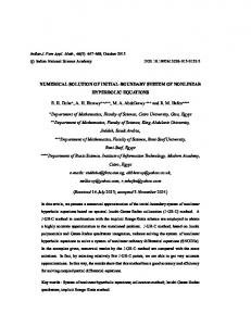
Consider each coordinate separately: introducing the partitions 0 = x0 < x1 < x2 < · · · < xnx < xnx +1 = 1, 0 = y0 < y1 < y2 < · · · < yny < yny +1 = 1 of [0, 1], we define the grid (tensor product grid) or mesh Ωh := (xi , yj ) : 0 ≤ i ≤ nx + 1, 0 ≤ j ≤ ny + 1 consisting of (nx + 2)(ny + 2) points. A grid which is equidistant (in both directions) is one in which the grid spacing in each direction is constant: xi = i∆x,

i = 0, 1, . . . , nx + 1,

∆x = 1/(nx + 1),

yj = j∆y,

j = 0, 1, . . . , ny + 1,

∆y = 1/(ny + 1).

For equal spacing in both directions (uniform grid) we set we set h := ∆x = ∆y. 5.1 Laplace’s Equation on a Square


191


1

1

0.8

0.8

0.6

0.6

0.4

0.4

0.2

0.2

0

0

0

0.2

0.4

0.6

0.8

tensor product grid


1

0

0.2

0.4

0.6

0.8

1

equidistant grid


192


1

0.8

0.6

In the following we consider the uniform case ∆x = ∆y = h.

0.4

0.2

0

0

0.2

0.4

0.6

0.8

1

uniformes Gitter



193


Notation: ui,j := u(xi , yj )

function value of exact solution at point (xi , yj )

Ui,j ≈ ui,j

approximation of u(xi , yj ).

Taylor-expansion at (xi , yj ): 2 3 4 h h h ui+1,j = ui,j + hux + uxx + uxxx + uxxxx + O(h5 ), 2 6 24 i,j h2 h3 h4 ui−1,j = ui,j + −hux + uxx − uxxx + uxxxx + O(h5 ), 2 6 24 i,j

Summing yields (the terms with h5 also cancel) 4 h + O(h6 ). ui+1,j + ui−1,j = 2ui,j + h2 uxx + uxxxx 12 i,j



194


Analogously, in the y-direction, 4

ui,j+1 + ui,j−1 = 2ui,j + h2 uyy +

h uyyyy 12

+ O(h6 ) i,j

and, summing all 4 expansions and dividing by h2 , ui+1,j + ui−1,j + ui,j+1 + ui,j−1 − 4ui,j = 2 h | {z }

h2 ∆u + (uxxxx + uyyyy ) +O(h4 ). 12 i,j

=:(∆h u)i,j

The difference formula ∆h is called the 5-point-stencil or 5-point discrete Laplacian. Summary: In each grid point (xi , yj ), ∆h approximates the Laplace operator with a local discretisation error of order O(h2 ) as h → 0, i.e., (∆h u)i,j = (∆u)i.j + O(h2 ). Note: This requires sufficient smoothness of the solution, in this case u ∈ C 4 (Ω). 5.1 Laplace’s Equation on a Square


195


In analogy with the differential equation (5.1a) we now require that the approximate solution Ui,j satisfy the discrete Laplace equation ∆h Ui,j := (∆h U )i,j = 0,

1 ≤ i ≤ nx , 1 ≤ j ≤ ny .

(5.2a)

(5.2a) represents nx ny equations in (nx + 2)(ny + 2) unknowns, since the 5-point stencil is not applicable in the boundary points. But there, the boundary conditions supply the missing equations: Ui,j = g(xi , yj )

if (xi , yj ) ∈ ∂Ω.

(5.2b)

Written out in detail, (5.2b) reads U0,j = g(0, yj ),

Unx +1,j = g(1, yj ),

0 ≤ j ≤ ny + 1,

Ui,0 = g(xi , 0),

Ui,ny +1 = g(xi , 1),

0 ≤ i ≤ nx + 1.



196


Taken together, equations (5.2) represent a linear system of equations (5.3)

Au = f

to determine the (unknown) approximate values Ui,j at the interior grid points. The entries of the coefficient matrix A and right hand side f depend on our enumeration of the unknowns. A common one is the lexicographic order: u = [U1,1 , U2,1 , . . . , Unx ,1 , U1,2 , . . . , Unx ,2 , . . . , U1,ny , . . . , Unx,ny ]> or 

u1



   u2    u =  . ,  ..    uny 5.1 Laplace’s Equation on a Square

 where

U1,j



   U2,j    uj =  .  ,  ..    Unx ,j

j = 1, 2, . . . , ny .


197


Die Matrix A possesses the block structure  T I  I T I  1  .. .. . . A= 2 I  h  ..  . I  I in which I denotes the nx × nx  −4 1   1 −4   T = 1    

     ∈ Rnx ny ×nx ny ,    

T

identity matrix and T is the tridiagonl matrix  1 ..

.

..

.

..

. 1

1 5.1 Laplace’s Equation on a Square



     ∈ Rnx ×nx .    

−4 TU Bergakademie Freiberg, SS 2012

198


For unknowns Ui,j near the boundary, i.e., i = 1, nx

or

j = 1, ny ,

the 5-point stencil (5.2a) contains neighboring approximation values already specified by the Dirichlet boundary condition (5.2b). Moving these to the right hand side of each corresponding equation, we obtain for the (nonzero) entries of the vector f in (5.3) for the example shown f3,3

1 = − 2 g(x3 , y4 ) + g(x4 , y3 ) h

or

f2,1

1 = − 2 g(x2 , y0 ), h

respectively.



199


Due to the • simple geometry of Ω, • the simple structure of the Laplacian and • the same type of boundary conditions on all boundaries, the block tridiagonal matrix A possesses additional structure: it can be built up from discretisation matrices arising in the simpler one-dimensional BVP. We therefore consider the discretization of the (ordinary) one-dimensional BVP u00 (x) = 0, u(0) = g0 , u(1) = g1 using central differences with uniform mesh width h = 1/(n + 1).



200


Its discrete approximation leads to the linear system of equations A ∈ Rn×n , f ∈ Rn ,

A1 u = f , where 

−2

  1 1 1   A1 = 2 tridiag(1, −2, 1) := 2  h h  

1 .. . .. .

 ..

   ,   

. 1

1

−2

  g0   0   1  ..   f =− 2. h    0   g1

and vector of unknowns u = [U1 , U2 , . . . , Un ]> ,


Ui ≈ u(xi ),

i = 1, 2, . . . , n.


201


The discretization of the two-dimensional Laplace operator can now be expressed as A = T1 ⊗ I + I ⊗ T1 (5.4) with T1 =

1 h2

tridiag(−1, 2, −1).

In equation (5.4), the Kronecker product (or tensor product) M ⊗ N of two matrices M ∈ Rp×q and N ∈ Rr×s is defined by   m1,1 N . . . m1,q N  .  .  ..  ∈ Rpr×qs M ⊗ N =  ..  mp,1 N . . . mp,q N and I is the identity matrix in Rn .



202


5.1.2

The Neumann Problem

We now consider a BVP for the Laplace operator in which the Dirichlet BC are replaced by the Neumann BC ∂u = h(x), ∂n

x∈Γ

(5.5)

Since in our model problem the four segments of the boundary Γ of the domain Ω lie parallel to the coordinate axes, the discretization of (5.5) is easy. In the boundary points (x0 , yj ), for example, one may use either U0,j − U1,j = h(x0 , yj ), h U−1,j − U1,j = h(x0 , yj ) 2h

(backward difference),

(5.6a)

(central difference)

(5.6b)

with analogous formulas at the remaining boundaries. 5.1 Laplace’s Equation on a Square


203


Note: • The central difference formula (5.6b) introduced so-called ghost points U−1,j , which, strictly speaking, lie outside the domain Ω. These can, however, immediately be eliminated from the equations by solving (5.6b) for U−1,j and inserting this expression into the 5-point stencil centered at (x0 , yj ). • In contrast to the discretized Dirichlet problem with the same mesh width h, for the Neumann problem the unknowns Ui,j on the domain boundary Γ are not fixed by the boundary conditions alone, but must also be determined, along with the interior unknowns, by solving the coupled linear systyem of equations. In this case the system has (nx + 2) · (ny + 2) unknowns.



204


The discretization matrix (same ordering) is now obtained as the Kronecker product A = Te1 ⊗ I + I ⊗ Te1 with  −1   1  1  Te1 = 2  h    



1 −2

..

.

..

.

..

.

−2 1


     .   1  −1


205


5.1.3

Eigenvalues and Eigenvectors

One of the reasons why (5.1) is often chosen as a model problem is that the spectral decomposition of the discretization matrix is available in closed form. Beginning with the n × n matrix T1 = h12 tridiag(1, −2, 1), we have T1 vj = λj vj ,

j = 1, 2, . . . , n,

with eigenvalues λj =

2 4 2 jπh [cos(jπh) − 1] = − sin , 2 2 h h 2

and (orthonormal) eigenvectors r 2 [vj ]k = sin(jkπh), n+1


j = 1, 2, . . . , n,

(5.7)

k = 1, 2, . . . , n; j = 1, 2, . . . , n.


206


Using properties of the Kronecker product of matrices, the eigenvalues and eigenvectors of the 2D problem can also be inferred from those of the 1D problem. More precisely: the eigenvalues λi,j of A in (5.4) are given by λi,j = λi + λj ,

1 ≤ i, j ≤ n,

(5.8)

with associated eigenvectors vi,j = vi ⊗ vj ,


1 ≤ i, j ≤ n.


207


5.1.4

Stability and Convergence

As we have already shown in the derivation of the 5-point approximation ∆h of the Laplace operator, there holds ∆h ui,j = ∆ui,j

h2 + (uxxxx + uyyyy )i,j + O(h4 ). 12

Setting [dh ]i,j := ∆h ui,j − ∆ui,j

(local discretization error)

[eh ]i,j := ui,j − Ui,j

(global discretization error)

we conclude that, due to ∆u = 0 for the exact solution u of the BVP, eh solves the linear system of equations Ah eh = dh = O(h2 ) with Ah = A the matrix in (5.4). 5.1 Laplace’s Equation on a Square


208


We therefore have eh = A−1 h dh and, because of −1 keh k = kA−1 d k ≤ kA h h h kkdh k

the O(h2 ) behavior as h → 0 is transferred from the local to the global discretization error if kA−1 h k remains uniformly bounded for all sufficiently small values of h > 0. Fixing the norm to be the Euclidean norm k · k = k · k2 , we have kA−1 h k

1 . = |λmin (Ah )|

The uniform boundedness property can now be inferred from (5.7) and (5.8), since 4 2 πh |λmin (Ah )| = 2 · 2 sin = 2π 2 + O(h2 ), h 2


(h → 0).


209


Summary: The (global) discretization error of the approximate solution of the model problem (5.1) obtained by finite difference approximation using central differences with uniform mesh size h satisfies keh k = O(h2 )

as h → 0,

assuming the solution u is four times continuously differentiable. The uniform boundedness of kA−1 h k as h → 0 is a stability property of the difference scheme.



210


5.1.5

The Poisson Equation

Replacing the Laplace equation (5.1a) in the BVP (5.1) by the inhomogeneous equation ∆u = f (Poisson equation), (5.9) with a given function f = f (x, y) defined on Ω, applying the central finite difference discretization leads to the discrete problem in which (5.2a) is modified to ∆h Ui,j = fi,j ,

with

fi,j = f (xi , yj ),

1 ≤ i ≤ nx , 1 ≤ j ≤ ny .

For the Dirichlet problem, the right hand side f of the resulting linear system of equations (5.3) consists of the sum of the Dirichlet boundary values and the corresponding function values fi,j .



211


5.1.6

The 9-Point Stencil

Since the formulas for difference schemes such as ∆h u can become cumbersome, particularly in 2 or more space dimensions, the following notation, in which the weights defining the scheme are given in a table corresponding to their spatial arrangement, is sometimes practical:   0 1 0  1   ∆h , 2 1 −4 1 . h 0 1 0 Using this notation, the approximation  1 1  (9) ∆h , 2  4 6h  1

4 −20 4

 1  4  1

of the Laplace operator is known as the 9-point stencil. 5.1 Laplace’s Equation on a Square


212


Using the same analysis based on Taylor series expansion reveals that (9) ∆h u

h2 = ∆u + (uxxxx + 2uxxyy + uyyyy ) + O(h4 ). 12 (9)

As an approximation of ∆, the 9-point stencil ∆h therefore has the same order of consistency as the 5-pont stencil ∆h . However, it can still be used to construct a higher order approximation as follows: The leading error term is observed to contain the biharmonic operator applied to u: uxxxx + 2uxxyy + uyyyy = ∆(uxx + uyy ) = ∆(∆u) = ∆2 u.



213


Since the exact solution u of the Poisson equation satisfies ∆u = f , we can conclude that the local discretization error of the approximate equation (9) ∆h Ui,j = fei,j ,

1 ≤ i ≤ nx , 1 ≤ j ≤ ny ,

with the modified right-hand side 2 h fei,j := f (xi , yj ) + ∆f (x, y) 12

has order O(h4 ) as h → 0.



214


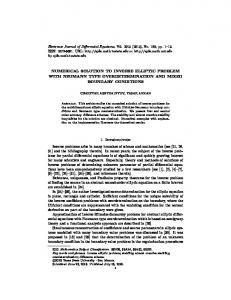
Example: We consider (cf. Section 11.4) the Poisson equation ∆u = −1 on Ω = (−1, 1)2 with homogeneous Dirichlet BCs. We discretize the problem (9) using both ∆h and ∆h and compare the absolute value of the error in the point (0, 0) for different values of the mesh size h. (9)

n×n

∆h

7×7

3.6e − 03

1.8e − 05

15 × 15

9.0e − 04

1.1e − 06

ï2

10

∆h

2.3e − 04

7.0e − 08

63 × 63

5.7e − 05

4.3e − 09

127 × 127

1.4e − 05

2.7e − 10

255 × 255

3.5e − 06

1.7e − 11

ï4

10

Error in (0,0)

31 × 31

5ïpoint stencil 9ïpoint stencil

ï6

10

ï8

10

ï10

10

ï12

511 × 511

8.9e − 07

1.4e − 12

10

0

10

1

2

10 10 Number of grid points in each direction

3

10

Note: The last problem requires solving a linear system of dimension 261,121 and takes 5s on a 3 year old laptop. 5.1 Laplace’s Equation on a Square
