the 2D orthogonal views along the orientations; and (3) measure the similarity ..... be in an arbitrary position, so some affine transformation can be taken to simplify this .... w s k w. = = = â. = â. â. (3) where wi is the weight of view i, the other ...
A 3D Model Retrieval Method Using 2D Freehand Sketches Jiantao Pu, Kuiyang, Lou, Karthik Ramani Purdue Research and Education Center for Information Systems in Engineering (PRECISE), Purdue University, West Lafayette IN 47907-2024
Abstract A method is proposed in this paper to retrieve desired 3D models by measuring the similarity between user’s sketches and 2D orthogonal views generated from 3D models. The proposed method contains three steps: (1) determinate the orientation of 3D model; (2) generate the 2D orthogonal views along the orientations; and (3) measure the similarity between user’s sketches and the 2D views. For these purposes, three respective algorithms are proposed. Users can submit one, two or three views intuitively as a query, which are similar to the three main views in engineering drawing. The weight of each sketch view can be reconfigured by users to emphasize its importance. It is worth to point out that our method only needs three or six views, while 13 views is the minimum set that have been reported by other researchers. A prototype system is developed to evaluate the validity of this proposed method. Key Words: 3D model retrieval, similarity measurement, sketch, user interface
1 Introduction 3D models are playing an important role in many mainstream applications such as industrial manufacture, games, biochemistry, E-business, art, and virtual reality. Many methods have been proposed to retrieve the desired models quickly and accurately from a database. These methods can be classified into four categories: (1) Feature-vector based method. Since a 3D shape can be described by some global geometric properties, such as volume, surface area, concentricity, curvature, and inertial moment, the similarity between arbitrary shapes will be measured by computing the distance between these feature vectors. Elad et al. [1] use moments to describe shape features that can be used to measure the similarity between 3D models. Suzuki [2] employs a combination of several features to search 3D models in a web-based retrieval system. Zhang et al. [3] propose a new set of region-based features for 3D models. Vranic et al. [4] suggest a method in which the feature vector is formed by a complex function on the sphere. Kazhdan et al. [5] introduce a new reflective symmetry descriptor to represent a 3D model’s shape feature. The advantage of this new descriptor is that it can describe global properties of a 3D shape. There are some other methods that use other high-level shape features, such as generalized cylinders [6], superquadrics [7], and geons [8]. However, when a large number of feature descriptors are used for the query, the system cannot respond quickly because tremendous computations are needed. (2) Statistics-based method. To overcome the limitation mentioned above, some statistics-based methods have been proposed and they describe a 3D shape by computing the distribution of some specified feature. Ankerst et al. [9] describe a method that characterizes the area of intersection with a collection of concentric
spheres. The similarity is measured by computing the L2 difference of two area distributions. Paquet et al. [10] present an approach for 3D model retrieval using the distribution of moment, normal, cord, color, material, and texture. Horn et al. [11] represent a 3D model in terms of its distribution of surface normal vectors. They align the Extended Gaussian Images (EGI) for each model based on its principal axes, and then compare two aligned EGIs by computing their L2 difference. Robert et al. [12] propose a new method to represent the features of an object as a shape distribution sampled from a shape function measuring global geometric properties of an object. It is simpler than other shape matching methods that require pose registration, feature correspondence, or model fitting. The statistical based method is not only fast and easy to implement, but also has some desired properties for practical applications, such as robustness and invariance. However, these methods are not sufficient to distinguish between similar classes of objects due to the fact that local shape features are not depicted explicitly. (3) Topology based method. A complex object can be regarded as an arrangement of simple primitives, or components [13]. Hilaga et al. [14] propose a topology matching method, in which the similarity between polyhedral models is calculated by comparing Multi-resolutional Reeb Graphs (MRGs). A MRG is the search key for 3D shape, and it is constructed by using a continuous function, such as geodesic distance. Su et al. [15] also use geodesic distance to establish a Reeb graph, and apply a concept of matching significant node in Reeb graph matching. Siddiqi et al. [16] present a shape description based on shock graph. The space of all such graphs can be characterized by the rules of a shock graph grammar. Sundar et al. [17] describe a method that encodes the geometric and topological information in the form of a skeletal graph and use graph-matching techniques to match the skeletons. Topology-based methods have many desired properties, such as intuitiveness, invariance, generality, and robustness. In the form of skeleton, not only global features but also local features are depicted. It is convenient for users to specify the desired part that they would like to match. However, this method requires a consistent model of an object’s boundary and interior, and it isn’t easy to register two skeletons robustly. (4) Image-based method. The human visual system has an uncanny ability to recognize objects from single views, even when presented monocularly under a fixed viewing condition. Cyr et al. [18] adopt a concept named aspect graph to group all views and represent a 3D object with a minimal set of 2D views. However, it has to determine the view transitions named visual events precisely; otherwise, a large number of views are needed. In a 2D sketch based user interface, Funkhouser et al. [19] propose an algorithm that matches 2D sketches with the views of 3D objects. 2D sketches are drawn with a pixel paint program, while 3D objects are represented by a series of 2D projections. They use Fourier transform to measure the similarity between sketches and rendered views. However, 13 thumbnail images with the boundary contours of a 3D object as seen from 13 orthographic view directions must be preprocessed.
In this paper, we propose a method to retrieve 3D models by measuring the similarity between user’s sketches and 2D orthogonal views generated from 3D models. The basic idea arises from such a fact (as Figure 1 shows): engineers usually express their concept of a 3D shape with three 2D views without missing any information. In the aspect graph based method [18], although the viewing space is portioned into a set of views, there are still many views. In the 2D sketch-based query method [19] proposed by Funkhouser et al., 13 thumbnail images from different view directions have to be preprocessed offline. In contrast with above two methods, our proposed method only needs three or six views that can be determined at real time. Front View
Side View Top View
Figure 1 Representation of 3D shape in engineering practice: Front view reflects the left-right and top-down relationships of the shape of 3D models; the top view the left-right and front-back relationships; and the side view the top-down and front-back relationships. The content of this paper is organized as follows. In Section 2, a maximum normal distribution method is presented to obtain an intuitive bounding box, whose sides and planes are used as the projection planes and directions. Section 3 describes the procedures to calculate the projected views of 3D polygon model along the respective projection plane and direction. To measure the similarity between 2D views, a 2D shape distribution method is proposed in Section 4. In Section 5, our prototype is described and some experiment results are presented to show the validity of this proposed method. Finally, the conclusion and future work are presented in Section 6.
2 Orientation Determination An intuitive way to determine projection planes and directions is to find a unique bounding box that encloses a three-dimensional model properly. The side directions can be regarded as the projection directions, while the surfaces as the projection directions. In many cases, a classical statistical method named principal component analysis (PCA) [20] is used to estimate the pose of 3D object. It is also known as the Karhunen-Loeve transform. The principal axes are eigenvectors associated with largest eigenvalues of 2nd order moments covariance matrix. PCA can find out the intuitive directions along which the mass is heavily distributed. However, it is not good enough at aligning orientations of different models within the same class, as Figure 2 shows. Extended Gaussian Image (EGI) [21] is another classical method to determine the orientation of 3D object. For a 3D object, each point on its Gaussian
MND Method
PCA Method
sphere corresponds to a particular surface orientation. The EGI extends the Gaussian sphere by placing a mass at each point on the Gaussian sphere, which is equal to the area of the corresponding face. In this way, a 3D shape is specified by representing area and orientation of the faces on a sphere. For two different convex objects, their EGI representations are determined uniquely. However, for nonconvex objects, different shapes may own the same EGI representation.
Figure 2 Orientation determination using PCA and MND methods for similar shapes To overcome this limitation, we propose a new orientation determination method. 3D shape is represented by a triple S={ pi | (Ni, Ai, Di), 0≤i≤n}, in which Ni represents the normal of polygon pi, Ai, represents the area, Di represents the distance between the mass center C and the polygon pi. In fact, Di can be the distance between any predefined point in 3D space and the polygon pi. In this paper, we adopt the mass center for the sake of simplicity. In the EGI method, only normals and surface areas are used to represent 3D shape. Our aim is to find out the normal along which the summed surface area is the largest and these surfaces have the same distance from the mass center. The basic steps are described as follows: (1) Compute the normal direction Nk for each triangle Δpkqkrk and normalize it. It is the cross product of any two edges: Nk =
pk qk × qk r k pk qk × qk r k
(1)
(2) Summarize the areas of all triangles with the same normals and same distance from the center mass. (3) Determine the three principal axes. The normal associated with the maximum areas is selected as the first principal axis bu. To get the next principal axis bv, we can search from the remaining normal distributions and find out the normal that satisfies two conditions: (a) with maximum areas; and (b) orthogonal to the first normal. Naturally, the third axis can be obtained by doing cross product between bu and bv: b w = bu × b v . (4) Find the center and the half-length of the bounding box. This can be done by
projecting the points of the convex hull onto the direction vector and finding the minimum and maximum along each direction.
MND Method
PCA Method
The bounding boxes shown in Figure 3 are some examples obtained by the MND method and PCA method respectively. It can be observed that the bounding boxes obtained by MND are more intuitive than those obtained by PCA.
Figure 3 Orientation determination using PCA and MND methods
3 2D Orthogonal View Generation Once the projection planes and directions are determined, the next step is to simulate the process when engineers express mechanical parts on a piece of paper. For 3D models represented in polygon mesh, four steps are adopted: Step 1: Initialization. A bounding box has six planes and directions. They are also the projection planes and directions. One way to represent projection planes and directions is to use some parameters illustrated by Figure 4, in which a projection plane is defined by (Pi, Ni) and the corresponding projection direction by Ni, where 1 ≤ i ≤ 6 , Pi and Ni are the center and normal of face i, respectively. (P2, N2)
(P3, N3)
(P1, N1)
Figure 4 Illustration of parameters for projection planes and directions. Step 2: Backface culling in object space. When engineers express 3D shape by 2D views, the invisible backfaces are often not taken into account. For polygon mesh, we adopt a generalized method as shown in Figure 5. To determine if a polygon is facing the camera, we need only calculate the dot product between the normal vector of that polygon and the vector from the camera to one of the polygon's vertices. If the dot product is less than zero, the polygon is facing the camera. If the value is greater than zero, it is facing away from the camera. Especially, for the case when the dot product is equal to zero, we regard it as visible because the side polygon will contribute the
final view. Figure 6(b) is the backface culling result for the model shown in Figure 8(a). Eye 90
=90
Figure 5 Back face culling in object space. Step 3: Inside edge culling. As shown in Figure 6(b), the processed result is still not ideal because the surface patches are composed of a series of triangles. To obtain the contour lines of 3D models, the inside edges have to be discarded. The inside edge has a distinguished property: it is shared by two polygons. With this definition, we can cull the inside edges completely by transcending all the triangles obtained after Step 2. Figure 6(c) is the result after the inside edge culling operation is carried out.
Eye (a)
(b)
(c)
(d)
(e)
Figure 6 Four steps for view generation: (a) an original 3D model; (b) after backface culling operation; (c) after inside face culling operation; (d) a view without occlusion culling; and (e) a simplified view of (d). Step 4: Orthographic projection transformation. This step is to project the remaining polygons onto the corresponding projection planes. However, the bounding box may be in an arbitrary position, so some affine transformation can be taken to simplify this process: (a) Define three right-hand orthogonal axes for the projection plane. Generally, projection direction can be regarded as the z-axis, while the two neighboring sides as the other axis that must satisfy the right hand rule; (b) translate the center of the projection plane to the origin (0, 0, 0); (c) align the projection direction with the z-axis, the other two axes with y-axis and x-axis; (d) transform the results back to the original position. To this point, a view along a certain direction can be generated, as shown in Figure 6(d). The views reflect the models’ complex inside structure precisely. However, due to the random property of the similarity measuring method explained in Section 4, this internal structure will lead to some negative impact on the retrieval discriminability,
especially for models with a complex internal structure, as shown in Figure 7. Furthermore, in many cases, the external shape is more desirable for users. To overcome this limitation, an additional Step 2.5 can be added between Step 2 and Step 3 to discard the occluded triangles completely.
(a) (b) (c) Figure 7 (a) and (b) are the two side appearance of the same model, (c) is the view with occlusion culling, (d) is the view with occlusion culling.
Step 2.5: Occluded triangle culling. This step is done by executing a series of fast ray-triangle intersection tests. For a reference triangle, select its center P1 as the starting point of one ray, and the projection direction as the direction of the ray. For all the triangles, calculate the intersection point P2 between this ray and the selected triangle. If the distance from P1 to P2 is larger than zero, then the reference triangle is visible, otherwise invisible. Repeat this test until all triangles are visited, then the occlusion culling operation is over. In Figure 7, (c) is the view without occlusion culling, while (d) is with occlusion culling. It can be seen that the latter are more concise In Table 1, some examples about view generation are shown. It can be seen that above methods can obtain good intuitive views from 3D models. Table 1 View generation examples 3D Model
Front View
Top View
Side View
4
2D Shape Distribution Method for Similarity Measurement
After the above steps, the 3D shape-matching problem is transformed into how to measure the similarity between 2D views, which can be illustrated by Figure 8. In the past, many methods [22, 23, 24] have been proposed to compute the similarity between two polygons, but they are not easily extended to the similarity measurement between views. In this paper, a 2D shape distribution method is derived on the basis of Robert et al.’s method [12] to measure the similarity between 2D views. It can be regarded as a kind of derivation from the 3D case. In other words, the similarity between views can be obtained by measuring their 2D shape distributions. Similar to the 3D case, the process to compute the degree of the similarity between 2D shapes is summarized as three steps:
(a)
(b)
Figure 8 Similarity measurement between freehand sketch (a) and 2D view generated from 3D Models (1) Uniform random sampling on view edges. The views are formed by a series of line segments. Some of them may overlap with each other. For the sake of convenience, we adopt a random sampling principal: select a line segment from the view randomly; then pick a point on the line segment randomly and save it into an array named S. During this process, the random generator plays an important role. It should has the ability to generate a random number greater than one million because we define one million samplings. But the system function rand() in the Windows platform can only generate a number less than 32768; therefore, we design a new random generator by using rand() twice: MyRand() = rand() × 32768 + rand(). (2) Shape distribution generation. The Euclidean distance between two random
sampled points is used to measure the shape features of polygons because other distance metrics are designed especially for 3D cases. By summarizing the numbers of point pairs with the same distance, the 2D shape distribution can be generated. Figure 9 shows the two distributions formed by the views in Figure 8. From the visual appearance, the two views are similar to some extent. The next step is to quantify this difference.
Figure 9 The two curves are the distribution of the two views in Figure 8 respectively. The horizontal axis represents the distance between two random points, while the vertical axis represents the number of the point pairs with the same distance. (3) Similarity measuring. Due to the fact that two different models may have a different size, a normalization step has to be taken to measure their difference on the basis of a common standard. Generally, two normalization methods are available: (a) align the maximum D2 distance values, and (b) align the average D2 distance values. For the first normalization method, the maximum values of the two shape distributions have to be adjusted to one same value, which is used to normalize the shape distribution. The other one is to use the mean value of distance to normalize the shape distribution. To alleviate the influence of high-frequency noise, we adopt the second one as the normalization standard. The similarity between the two views can be obtained by calculating the difference between their distributions in the form of histogram: n
Similarity = ∑ ( si − ki )2
(2)
i =0
where n is the divided histogram number of the shape distribution curve, and s and k is the probability at certain distance. The 2D shape distribution approach has the same advantages as the 3D case. It is simple and easy to implement, and also has some unique properties: (a) insensitive to geometric noise; (b) invariance to translation, rotation, and scaling; and (c) no need to find out the feature correspondences between models. To measure similarity between models that have multiple ortho-views, an additional step is needed to find out the correspondences between views of the two models. If the view generation step is carried out without the Step 2.5 in Section 4, then there are only three different views because the views generated from the positive and negative directions are the same. If the Step 2.5 is taken, then there are six different views in
which the projections along different directions are not the same because the internal structure is not taken into account. To determine the partnership of one view, we compare it with all the views of another model and select the most similar one as the corresponding view. In this way, the views from different models can be grouped into a series of pairs. By adding the similarities of these view pairs together, we can get the similarity between models.
5 Prototype System and Experimental Results 5.1 Sketch Based User Interface An intuitive application for this proposed method is sketch-based user interface, in which the query process is similar to that engineers represent 3D shape on a piece of paper. Figure 10 shows the user interface of our prototype system, users can express their concept intuitively. Their emphasis on some views can be realized by adjusting the weights.
Figure 10 The sketch based user interface of our prototype system The sketch based user interface that we design has the following properties: (1) Users can express their attention freely with no special instruction, since the most frequently chosen views are not characteristic views, but instead ones that are simpler to draw (front, side, and top views). (2) Users can also specify weights for certain views to emphasize the respective shape represented by this view. In this way, the similarity expressed in Equation (2) can be modified as n
Similarity = ∑ wi ( si − ki )2 i =0
n
∑w i =0
i
=1
(3)
where wi is the weight of view i, the other parameters are the same as Equation (2). If
one view has higher weight, then the shape that it describes will play a more important role to determine the similarity degree between two models. (3) The prototype system provides a feedback mechanism to allow users to retrieve 3D models from coarse to fine. 5.2 Performance Evaluation In order to evaluate its validity and performance, we have conduct some experiments and designed a database that contains more than 1,700 models from CAD domain and 1,841 models from Princeton’s benchmark library. We put all the models contained in twelve groups into a library and measure the retrieval accuracy by checking the probability that the models within the same group appear in higher similarity. Two retrieval examples are shown in Table 2, and the quantitative results are shown in Table 2, in which the retrieval efficiency is also recorded. For models of a different size, the computation time is different. Table 2 Two examples retrieved by sketches Sketches
Top Five Similar Models
Table 3 Retrieval performance of our proposed method Performance Manners
Top 5
Top 10
Average retrieval time (second)
Average accuracy (Percent: %)
(1) Invariance (2) Robust (3) Generality
Retrieval by 3D model
With occlusion culling
49.7%
72.5%
0.73~3.12
Yes
No occlusion culling
41.3%
69.6%
0.85~3.74
Yes
Sketch based retrieval
With weights
73.3%
84.2%
0.23~2.92
Yes
No weights
51.4%
77.5%
0.23~2.92
Yes
As Table 2 shows, the performance of sketch based retrieval is much better than that of query by 3D model directly. Similar to the case of occlusion culling, the sketched shape represents the most important information that users want to express. The shape distribution of a sketch can reflect that of the ideal 2D shape much better, as too rich details will influence the shape distribution to some extent. This is also the reason that
the retrieval performance with occlusion culling is better than that without occlusion culling. At the same time, it also shows that the retrieval accuracy can be surprisingly improved by modulating the weights of the three views properly. Users can retrieve the desired models by adjusting the weight values of views that they intend to emphasize.
6 Conclusion This paper presents a 3D model retrieval method by measuring the similarity between 2D views. This method enables the intuitive implementation of a 2D sketch user interface for 3D model retrieval. Users can submit one, two, or three sketches as a query and adjust the weight of each view to emphasize the search intention. The sketching way is very similar to the process that engineers express their design conception on a piece of paper. Because this method is based on some statistical information of 2D shape, the sketch user interface can provide a robust way that does not require a perfect sketch as query, and users can express their ideas freely without any fear of making mistakes. In the future, we will focus our attention on local shape matching, in which users can specify some local shape explicitly.
References [1] Elad, M., Tal, A., and Ar, S., “Content Based Retrieval of VRML Objects: An Iterative and Interactive Approach,” Proc. 6th Eurographics Workshop on Multimedia 2001, pp.107-118, Manchester, UK, 2001. [2] Suzuki, M.T., “A Web-based Retrieval System for 3D Polygonal Models,” Proc. Joint 9th IFSA World Congress and 20th NAFIPS International Conference (IFSA/NAFIPS2001), pp.2271-2276, Vancouver, 2001. [3] Zhang, C., and Chen, T., “Indexing and Retrieval of 3D Models Aided by Active Learning,” Proc. ACM Multimedia 2001, pp. 615-616 Ottawa, Ontario, Canada, 2001. [4] Vranic, D.V., and Saupe, D., “Description of 3D-Shape using a Complex Function on the Sphere,” Proc. IEEE International Conference on Multimedia and Expo (ICME 2002), pp.177-180, Lausanne, Switzerland, 2002. [5] Kazhdan, M., Chazelle, B., Dobkin, D., Funkhouser, T., and Rusinkiewicz, S., “A Reflective Symmetry Descriptor for 3D Models,” Algorithmica, 38(2): 201-225, 2003. [6] Binford, T.O., “Visual Perception by Computer,” Proc. IEEE Conference on Systems and Control, pp.183-193, 1971. [7] Solina, F., and Bajcsy, R., “Recovery of Parametric Models from Range Images: The Case for Superquadrics with Global Deformations,” IEEE Transactions on Pattern Analysis and Machine Intelligence, 12(2): 131– 147, 1990. [8] Wu, K., and Levine, M., “Recovering Parametric Geons from Multiview Range Data,” Proc. CVPR, pp.159–166, 1994. [9] Ankerst, M., Kastenmuller, G., Kriegel, H.P., and Seidl, T., “3D Shape Histogram for Similarity Search and Classification in Spatial Databases,” Proc. 6th International Symposium on Spatial Databases, pp.207-228, HongKong, China, 1999.
[10] Paquet, E., and Rioux, M., “Nefertiti: A Tool for 3-D Shape Databases Management,” SAE Transactions:Journal of Aerospace 108, pp.387–393, 2000. [11] Horn, B., “Extended Gaussian Images,, Proc. IEEE 72, 12(12), pp.1671-1686. New Orleans, USA, 1984. [12] Robert, O., Thomas, F., Bernard, C., and David, D., “Shape Distribution,” ACM Transactions on Graphics, 21(4): 807-832, 2002. [13] Biederman, I., “Recognition-by Components: A Theory of Human Image Understanding,” Psychological Review, 94(2):115-147, 1987. [14] Hilaga, M., Shinaagagawa, Y., Kohmura, T., and Kunii, T.L., “Topology Matching for Fully Automatic Similarity Estimation of 3D Shapes,” Proc. SIGGRAPH 2001, Computer Graphics Proceedings, Annual Conference Series, pp.203–212, Los Angeles, USA, 2001. [15] Su, L.S., and Lee, T.Y., “3D Model Retrieval using Geodesic Distance,” Proc. Computer Graphics Workshop, pp.16-20, Tainan, 2002. [16] Siddiqi, K., Shokoufandeh, A., Dickinson, S., and Zucker, S., “Shock Graphs and Shape Matching,” Computer Vision, 35(1): 13-20, 1999. [17] Sundar, H., Silver, D., Gagvani, and Dickinson, S., “Skeleton Based Shape Matching and Retrieval,” Proc. Shape Modeling International 2003, pp.130-142, Seoul , Korea, 2003. [18] Cyr, C.M., and Kimia, B.B., “3D Object Recognition Using Shape Similarity-Based Aspect Graph,” Proc. 8th International Conference On Computer Vision, pp.254-261, Vancouver, Canada, 2001. [19] Funkhouser, T., Min, P., Kazhdan, M., Chen, J., Halderman, A., Dobkin, D., and Jacobs, D., “A Search Engine for 3D Models,” ACM Transactions on Graphics, 22(1): 83-105, 2003. [20] Petrou, M., and Bosdogianni, P., “Image Processing: The Fundamentals,” John Wiley, 1999. [21] Horn, B.K.P., “Extended Gaussian Images,” Proc. IEEE, 72(12): 1671-1686, 1984. [22] Arkin, E.M., Chew, L.P., Huttenlocher, D.P., Kedem, K., and Mitchell, J.S.B., “An Efficiently Computable Metric for Comparing Polygonal Shapes,” IEEE Transactions on Pattern Analysis and Machine Intelligence, 13(3): 209-216, 1991. [23] Tung, L.H., and Irwin, K.F, “A Two-Stage Framework for Polygon Retrieval,” Multimedia Tools and Applications, 11: 235-255, 2000. [24] Avis, D., and Elgindy, H., “A Combinatorial Approach to Polygon Similarity,” IEEE Transactions On Information Theory, IT-29: 148-150, 1983.