3D Model Retrieval Based on Orthogonal Projections ﹡
Liu Wei , He Yuanjun Department of Computer Science and Engineering, Shanghai Jiaotong University, Shanghai, 200240, P.R.China
Abstract Recently with the development of 3D modeling and digitizing tools, more and more models have been created, which leads to the necessity of the technique of 3D mode retrieval system. In this paper we investigate a new method for 3D model retrieval based on orthogonal projections. We assume that 3D models are composed of trigonal meshes. Algorithms process first by a normalization step in which the 3D models are transformed into the canonical coordinates. Then each model is orthogonally projected onto six surfaces of the projected cube which contains it. A following step is feature extraction of the projected images which is done by Moment Invariants and Polar Radius Fourier Transform. The feature vector of each 3D model is composed of the features extracted from projected images with different weights. Our System validates that this means can distinguish 3D models effectively. Experiments show that our method performs quit well.
Key words: 3D model retrieval, orthogonal projections, moment invariants, fourier transform
1 Introduction Now 3D models play an important role in many applications such as computer game, computer aided design, e-business, molecular biology, cultural relic preservation, etc, and become the forth multimedia type after sound, image and video[1]. Recent developments in techniques for modeling, digitizing and visualizing 3D shapes have led to an explosion in the number of available 3D models on the Internet and in domain-specific databases. This has led to the development of 3D shape retrieval systems which can retrieve similar 3D objects according to the given query object. This problem involves many fields such as Computer Graphics, Artificial Intelligence, Computer Vision, Pattern Recognition, etc. The standard descriptions have been brought into the frame of MPEG-7[2]. 3D Model Retrieval based on content first automatically computes model data thus extract features such as shape, space relation, color and texture of material, etc, then establishes an index for multi-dimension information of 3D model. We can calculate the similarity between the query model and the aimed models in multi-dimension feature space so as to realize the browse and retrieval of 3D model database. Thus users can get their needed models using ocular feature matching, which is more close to the mode that people usually rely on their intuition and impression to use information in real life. _______________________________________ ﹡
Corresponding author: Tel: +86-(21)-34205230 Fax: +86-(21)-34204486 E-mail:
[email protected]
The outline of the rest of this paper is as follow: in the next section we review the relevant previous work. In Section 3 we describe feature extraction and comparison based on orthogonal projections. In Section 4 experiments and results are presented in detail. At last we give the conclusion and future work in Section 5.
2 Previous Work Paquet made the initial research and got remarkable achievements[3][4]. From then on, a lot of researches have been carried on. Now many approaches have been proposed In general, they can be divided into four types: Retrieval based on shape, Retrieval based on topology, Retrieval based on image and Retrieval based on surface attributes. Anderst[5] directly syncopated 3D model with some mode, then calculated the proportions of point number of each unit in that of the whole model, thus a shape histograms was formed. In his paper, Anderst introduced three methods to syncopate 3D models: shell model, sector model and spider web model. So we can retrieve model through comparison of shape histograms. Suzuki[6] put forward to a different method to syncopate 3D models which was called point density. This method did not form feature vector only by the syncopated units but classified the syncopated units, so the dimension of feature vector and computational quantity decreased greatly. Osada[7] investigated a 3D model retrieval system based on shape distributions. The main idea was to calculate and get large numbers of statistical data which could be served as shape distributions to describe the features of models. The key step was to define the functions which could describe the models. Reference [7] defines five simple and easy-to-compute shape functions: A3, D1, D2, D3 and D4. Because this method was based on large number of statistical data, it was robust to noise, resampling and mesh simplification. Vranic’s[8] method firstly voxelized the 3D model, then applied 3D Fourier Transform on these voxelizations to decompose the model into different frequencies, finally choosed certain amount of coefficients of frequency as this model’s feature vector. Another approach[9] investigated by Vranic was spherical harmonics analysis, which was also called 2D Fourier Transform on unitary sphere. This method needed sampling and harmonics transform, so the process of feature extraction was slow. Chen[10] had developed a web-based 3D model retrieval system in which a topology method using Reeb graph was introduced. Reeb graph could be constructed by different precisions, thus in this way mutli-resolution retrieval was available. There are also many searches on image-based retrieval[11] [12] [13],of which Chen at Taiwan University made outstanding productions[12]. In Chen's system, several images, taken from different views around, are used to represent a 3D model and then transformed into descriptors. Thereafter, the matching of any two 3D models is achieved by matching two groups of 2D images by those descriptors. 100 images which belong to 10 lightfields for each model are required and the calculation is enormous. The method proposed in the paper also belongs to this type but aims to reduce the number of images required for per 3D model, thus quickens the speed of retrieval.
3 Feature Extraction and Comparison The essence of 3D model retrieval is comparison of feature vectors, so the choice of feature is vital to the performance of a 3D model retrieval system. In this paper, we propose a method based on orthogonal projections and the process of feature extraction and comparison can be divided into four steps as follow: 1. Normalize the pose; 2. Project the 3D models onto six surfaces of the
projected cube; 3. Extract features of the projected images; 4. Compare the 3D models. The rest of the section will discuss the above four steps one by one in detail.
3.1 Pose Normalization 3D models have arbitrary position, orientation and scaling in 3D space. In order to capture the projected features of a model, the model has to be placed in a canonical coordinate frame. Thereby, if we scaled, translated, rotated or flipped a model, then the placing into the canonical frame would be the same. Let P = {P , P L P }( P = ( x , y , z ) ∈ R3 be the set of vertices on the surface of this model. 1 2
m
j
j
j
j
The goal of pose normalization is to find an affine map
τ : R 3 → R 3 in such a way that a
model of any translation, rotation and scaling can be put normatively by this transformation. The translation invariance is accomplished by finding the center of the model: 1 m −1 1 m −1 1 m −1 x = x,y = y ,z = z ∑ ∑ c m i c m x c m ∑ i i=0 i=0 i=0
So the point P ( x , y , z ) is the center of this model, we move P
c
Thus
for
each
c
point
c
c
c
P = (x , y , z ) ⊂ P , j j j j
a
to coordinate origin.
corresponding
transformation:
P ' = ( x − x , y − y , z − z ) is performed. Based on the transformation we define points set j j c j c j c
P ' = {P ' , P ' , L , P ' } . 0 1 m The rotation invariance is accomplished by the method of PCA(Principle Component Analysis). We calculate the covariance matrix C . ⎡m 2 ⎢∑ x ⎢ km= 0 m T C = ∑ Pk Pk = ⎢∑ xy ⎢k =0 k =0 ⎢m ⎢ ∑ xz ⎣⎢ k = 0
m
m
⎤
∑ xy ∑ xz ⎥ ⎥ ⎥ yz ∑ ⎥ k =0 k =0 m m ⎥ 2 yz ∑ z ⎥ ∑ k =0 k =0 ⎦⎥ k =0 m
∑y
k =0 m
2
This step must be done after the translation of Pc to coordinate origin. Obviously the matrix C is a real symmetric one, therefore its eigenvalues are non-negative real numbers. Then we sort
the eigenvalues in a non-increasing order and find the corresponding eigenvectors. The eigenvectors are scaled to Euclidean unit length and we form the rotation matrix R which has '
the scaled eigenvectors as rows. We rotate all points in P and a new points set is formed:
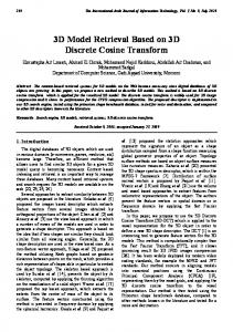
P ' ' = {P ' ' | P ' ' = P ' R, P ' ∈ P i , l = 0, L, m) l l l l When this step has been done, the model is rotated so that the X-axis maps to the eigenvector with the biggest eigenvalue, the Y-axis maps to the eigenvector with the second biggest eigenvalue and the Z-axis maps to the eigenvector with the smallest eigenvalue[14]. An effect of PCA is
illuminated as Figure 1, the left model is in a gradient coordinate frame while after PCA it is placed regularly as showed in the right image.
Fig.1. An effect of PCA
The scaling invariance is accomplished by zooming in or out the model to a fixed size. Firstly let rmax be the max distance from the set of vertices to coordinate origin. Next for each point in
P ' ' ,we must do the third transform and obtain the final points set:
x'' ' ' ' P = {( s
r max
y'' , s
r max
Obviously, for each point in P
z'' , s
r max
) | ( x ' ' , y ' ' , z ' ' ) = P ' ' ∈ P ' ' , s = 0, L , m} s s s s
' ' ' , the following inequation come into existence.
− 1 ≤ x ' ' ' , y ' ' ' , z ' ' ' ≤ 1, ( x ' ' ' , y ' ' ' , z ' ' ' ) = p ' ' ' ∈ P ' ' ' , t = 0,L , m t t t t t t t So the model can be contained in a cube whose center is coordinate origin and length of arris is 2, we call such a cube axis-aligned bounding box(AABB). The new model which is composed '''
of points set P and has the same topology structure as the original model is just the result of process of pose normalization. We must notice that the distribution of points may not be uniform, for example, a large quadrangle in the surface of a model can be decomposed into two triangles and four points while some fine detail needs hundreds of triangles and points. Thus the result of pose normalization will not be perfect. We can easily modify the method described above. A feasible way is that the points set P is taken uniformly from the surface of a model instead of the original set of vertices. Detailed introduction about uniform point-taking can be found in Reference [15].
3.2 Project the 3D Models onto Six Surfaces of AABB After the pose normalization has been done, we can project the 3D model onto the planes and form 2D images. The planes we chose are the six surfaces of the projected cube. The main idea is to divide the model according to the three orthogonal planes of Cartesian reference frame: XY-plane, YZ-plane and ZX-plane and each plane divides the model into two parts. Figure 2 shows the division. Notice that the images on two parallel projected planes are different if the model is not symmetrical with regard to the corresponding syncopating plane.
Fig.2. Syncopating Planes
To illustrate the difference of distances from the points on the surface of the divided model to the projected planes, we use different gray values on the projected 2D images. The bigger the distance is, the bigger gray value the corresponding projected point has. Figure 3 shows the result of the projections of the model of insect as showed in Figure 1. The projected images is fixed to 256 × 256 and the process of projection can be achieved by Z-buffer arithmetic[16]. For some models, the projected images have spiculate edges and corners, which make it hard for further process, so a step to smooth the projected images is necessary. In this paper, we adopt the mean of Dilation in Mathematical Morphology[17] to achieve the aim.
Fig.3. Projections
3.3 Feature Extraction of the Projected Images Now we have six projected images for each 3D model which are corresponding to the model, so the united features of these images also basically represent the features of the 3D model. Since the foreground and background of these projected images are clearly differentiated, the images needn’t segmentation and the extraction of feature becomes easy. In this paper, we join up two ways to enhance the performance of the arithmetic: Moment Invariants and Polar Radius Fourier Transform. These two approaches extract feature vectors respectively in space domain and frequency domain.
3.3.1 Moment Invariants Moment Invariant proposed by Hu[18] is a kind of feature based on region. Let f ( x, y ) be a 2D digital image with its size being M × N . The ( p + q ) rank central moment is defined as following:
m
M N p q = ∑ ∑ f (i, j )(i − x ) ( j − y ) , p, q = 0,1, L pq c c i=0j=0
( x , y ) is the centroid point of the image . Based on the definition above, Hu defined 7 c c moment invariants as:
u =m +m 1 20 02 u = ( m − m ) 2 + 4m 2 2 20 02 11 2 u = ( m − 3m ) + (3m − m ) 2 3 30 12 21 03 u = (m + m ) 2 + (m + m )2 4 30 12 21 03 u = ( m − 3m )( m + m )[( m + m ) 2 − 3( m + m ) 2 ] + (3m − m )( m + m )[3( m + m ) 2 − ( m + m ) 2 ] 5 30 12 30 12 30 12 21 03 21 03 21 03 30 12 21 03 u = ( m − m )[( m + m ) 2 − ( m + m ) 2 ] + 4m ( m + m )( m + m ) 6 20 02 30 12 21 03 11 30 12 21 03 u = (3m − m )(m + m )[( m + m ) 2 − 3( m + m ) 2 ] + ( m − 3m )( m + m )[3( m + m ) 2 − ( m + m ) 2 ] 7 21 03 30 12 30 12 21 03 30 12 21 03 30 12 21 03
The 7 moment invariants keep changeless to the translation, rotation and scaling of the object in the images. We can form a feature vector of an image using these 7 moment invariants. Because different moment invariants represent different physical meanings, they have different scopes of values and can not be compared directly. We must place these moment invariants at the same status so that these moment invariants play the same roles in comparison of feature vectors, Conference [19] introduces a method based on Gauss unitization.
3.3.2 Polar Radius Fourier Transform Polar Radius Fourier Transform is based on the contour. So the first step is contour extraction of the projected images. We used contour tracking arithmetic introduced in Conference [20]. The result is showed in Figure 4(a). As the points numbers on the contour are different, we can’t directly apply this transform. Firstly we must sample the contour and remain the same number of points. To hold details on the contour, we adopt a method of equidistance in which two adjoined sampling points have the same distances on the contour, as showed in Figure 4(b).
Fig.4. a) Contour
b)Sampling on contour
Figure 4(b) has 360 sampling points, we can obverse that its shape is very close to the contour. Calculate the polar radius ri of each sampling point.
r = ( x − x ) 2 + ( y − y ) 2 , i = 0,1, L , N − 1 i i c i c ( x c , y c ) is the centroid of contour and
N is the number of sampling. Then we can
calculate the Polar Radius Fourier Transform:
j 2πni 1 N −1 a = ), n = 0,1, L , N − 1 r exp( − ∑ n N i N i=0 We choose the first several coefficients as the high frequency part is not steady and changes drastically when the contour has even a slight difference. To get invariance for scaling, we choose
the following list as feature vector: [
a1
,
a0
a2 a0
,L,
a 21
].
a0
3.4 Comparison of 3D models The distance between two models can be obtained by combining the distances of corresponding projected images with different weights. There are six 2D images for one 3D model, but there they are in different statuses. In this subsection, we investigate a method to unite the feature vectors of six images into one.
3.4.1 Comparison with different weights According to Section 3.1, we can be acquainted that after PCA the eigenvector corresponding to the biggest eigenvalue becomes X-axis, the eigenvector corresponding to the second biggest eigenvalue becomes Y-axis and the third eigenvector becomes Z-axis. The theory of probability points out that the value of eigenvalue represents the density of distributing of points in the direction of corresponding eigenvector, so projections form different directions play different roles in comparison. As showed in Figure 3, we can get rough shape from the image projected on XY-plane while we can’t from image projected on YZ-plane, this is because the information supplied by different projections is not equal. Let D xy , D yz , D zx (each actually has two distances, but has the same weights) respectively represent distances of projections of the two models from three coordinate planes and EV x , EV y , EVz are the eigenvalues calculated in the process of PCA when calculating the query
model. Then we can define the distance between two models:
D=
EV x EV y D xy +
EV y EV z D yz +
EV z EV x D zx
Thus the image which contains more information accordingly plays a more important role in comparison, as a result the distance D can represent the difference of two models more closely.
3.4.2 Comparison of Projected Images As illustrated in Section 3.3, there are two kinds of feature vectors, and the computations of distances of both vector adopt Euclidean Distance. But according to statistical data we notice that the two kinds of distance have different range of values. In general, the distance of feature vector composed of moment invariants ranges from 0.0 to 10.0, while the feature vector composed of coefficients of Fourier Transform ranges from 0.0 to 0.5. Obviously, they can not be added together directly. A feasible way is to externally unitize the feature vectors and make their distances range between [0, 1] to the best of our abilities. In this paper, we assume that the distributions of feature vectors of both kinds accord with Gauss Distribution. For each kind of feature vector of image, the detailed step to be externally unitized is as following: 1. Calculate all the distances between the same oriented projections of two models: Di, j , i , j = 1, 2 L , NUM , i ≠ j , NUM is the number of models in model database.
2. Calculate the average Daver and covariance σ of the NUM ( NUM − 1) 2 distances.
Daver and σ
are the inherent physical measure of a 3D model database and stay
invariable if the database remains changeless. So although the two steps above are very time-consuming, this work is once and for ever. 3. When we calculate D xy , D yz , or D zx , if Dimg is the preliminary result, then
Dimg = (
Dimg − Daver 3σ
+ 1) 2 .We can easily know that the probability of the fact that Dimg
falls into the range of [0,1] is over 99%. Thus we can add the two unitized distances directly. If we want to emphasize one of the two factors, we can endow it with a bigger weight.
4 Experiments and Results According to the method described above, we have developed a 3D model retrieval system using Visual C++. The system consists of off-line pre-process module and on-line retrieval process module. In the off-line pre-process, features of 3D models are extracted and stored in database within about 2 seconds on average for per model using a PC with Pentium IV 1.8G CPU and Windows 2000 Server Operation System. In the on-line process, users can select a 3D model as the query model and get the first 48 models which are most similar to the input one. A query needs 1.8 seconds on average. Figure 5 shows a typical example for a query of dogs. The left six images are the abbreviative projected images of the dog model. In this query, the weights of Moment Invariants and Polar Radius Fourier Transform are respectively 0.3 and 0.7. We can observe that the result is satisfactory.
Fig.5. A query of dogs
We have collected 2863 models from Web in total with a median of 3789 points and 7146 triangles per one. The models are not all well defined trigonal meshes,many of which contain cracks, self-intersections, polygons-missing, etc. To fairly test the performance, we use the Princeton Shape Benchmark (PSB), which is a defacto criterion of 3D model database and is introduced in Conference [21] in detail, to test our system. It is a collection of 1814 models which are manually divided into 161 classes, each containing at least 4 models. The performance can be decided by two measures: precision and recall. “Precision” measures that the ability of the system to retrieve only models that are relevant while “recall” measures the ability of the system to retrieve all models that are relevant. Let C be the number of relevant models in the database, in
other words, C is the number of models of the class to which the query model belongs. Let N be the number of relevant models that are actually retrieved in the top A retrievals. Then, recall and precision are defined as follows:
precision = N
A
, recall = N
C
There is a trade-off relationship between precision and recall. In our system each model has a feature vector of 162 dimensions. We test various kinds of models including animals, plants, cars, characters, and so on, from each kind we choose ten models as the query models and test the results. From the average precision-recall diagram, as showed in Figure 6, we can easily observe that Chen’s method only slightly outperforms ours, but the queries using our method is much quicker than his because ours need only fewer images to be compared despite that ours need an additional step of pose normalization.
Fig.6. Comparison of two methods
5 Conclusion and Future Work In this paper, we present a new 3D model retrieval system based on orthogonal projections. The contribution of this paper can be summarized as: Realize 3D model retrieval by 2D image comparisons and get considerable result at preferable speed. To improve the performance, we use two kinds of features to work together. At the same time, because our system is based on projections, we can easily realize the retrieval by 2D image. Given a 2D silhouette, we can get the models which have the similar silhouette. Furthermore, our method is robust to some kinds of flaws of 3D models as described in Section 4. The technology of 3D model retrieval is just underway and there is a long way to advance. Because of its complexity, many ripe methods which can be applied on images can not directly be transplanted to 3D models, as a result, the performance is not satisfactory on the whole and needs further enhancement. A next work of us is to apply the newest field in Digital Geometry Processing on the 3D model retrieval, the main idea being each model can be decomposed into a basal mesh and several details[22], then through analyzing these comparatively simple parts, we can obtain the firsthand features of 3D models.
Acknowledgements This research has been funded by The National Nature Science Foundation of
China (60573146) and The National High Technology R&D Program (863) for CIMS of China (2003AA411310).
References [1] Zhang Biqiang, Xun Yuan, Yuan Xueyu. Fast Generation of the Topological Information in STL for Mesh Simplification. Journal of Shanghai Jiaotong University, 2004, 38(1): 39-42 [2] Cui Chenyang, Si Jiaoying. Analysis of Feature Extraction in 3D Model Retrieval. Journal of Computer Aided Design and Graphics, 2004, 16(1): 882-889 [3] Paquet E, Rioux M. A query by content software for three dimensions database management. Proceeding of International Conference on Recent Advances in 3D Digital Imaging and Modeling, Ottawa, Canada, 1997, 345-352 [4] Paquet E, Rioux M. A content-based search for VRML database. Proceeding of the 1998 Computer Society Conference on Computer Vision and Pattern Recognition, Santa Barbara, CA, 1998, 541-546 [5] Ankerst Mihael, Kastenmller Gabi, Kriegel Hans Peter. 3D Shape Histograms for Similarity Search and Classification in Spatial database. Proceeding of the 6th International Symposium on Large Spatial Database, Hong Kong, 1999, 207-226 [6] Suzuki Motofumi T, Kato Toshikazu, Otsu Nobuyuki1. A Similarity Retrieval of 3D Polygonal Model Using Rotation Invariant Shape Descriptors. Proceeding of IEEE International on Systems, Man, and Cybernetics, Nashville, Tennessee, 2000, 2946-2952 [7] Osada Robert, Funkhouser Thomas, Chazelle Bernard. Shape Distributions. ACM Transactions on Graphics, 2002, 21(4): 807-832 [8] Vranic D V, Saupe D. 3D Shape Descriptor Based on 3D Fourier Transform. Proceeding of the EURASIP Conference on Digital Signal Processing of Multimedia Communications and Services, Budapest, Hungary, 2001, 271-274 [9] Vranic D V, Saupe D. Description of 3D Shape Using a Complex Function on Sphere. Proceeding of the IEEE International Conference on Multimedia and Expo, Lausanne, Switzerland, 2002, 177-180 [10] Chen Dingyun, Ouhyoung Ming. A 3D Object Retrieval System Based on Multi-Resolution Reeb Graph. Proceedings of Computer Graphics Workshop, Taiwan, China, 2002, 16-20 [11] Min Patrick, Chen Joyce, Funkhouser Thomas. A 2D Sketch Interface for a 3D Model Search Engine. Computer Graphics Proceedings, Annual Conference Series, ACM SIGGRAPH 2002 Technical Sketch, San Autonio, Texas, 2002 [12] Chen Dingyun, Tian Xiaopei, Shen Yute. On Visual Similarity Based 3D Model Retrieval. Computer Graphics Forum, 2003, 22 (3): 223-232 [13] Jobst Loffler. Content-Based Retrieval of 3D Models in Distributed Web Databases by Visual Shape Information. IEEE International Conference on Information Visualization, London ,UK, 20001 82-87 [14] Vranic D V, Saupe D, Richter J. Tool for 3D-objects Retrieval Karhunen-Loeve Transfrom And Spherical Harmonics. IEEE 2001 Workshop Multimedia Signal Processing, Cannes, France, 2001 [15] Zheng Bochuan. Research of 3D Model Retrieval Based on Content. Dissertation for Master’s Degree, Zhejiang University, 2004: 18-20 [16] David F.Rogers. Procedural Elements for Computer Graphics. China Machine Press, 2002
[17] Haralick R M, Sternberg S R, Zhuang Xinhua. Image Analysis Using Mathematical Morphology. IEEE Transcation on PAM, 1987, 9(4): 243-251 [18] Hu M K. Visual Pattern Recognition by Moment Invariants. IEEE Transaction on Information Theory, 1962, (8): 179-187 [19] Liu Jin, Zhang Tianxu. The Generalization of Moment Invariants. Chinese Journal of Computer, 2004, 27(4): 668-674 [20] He Bin, Ma Tianyu, Wang Yunjian. Digital Image Processing Using Visual C++(2nd). Post and Telecommunications Press, 2002: 435-444 [21] Philip Shilane, Patrick Min, Michael Kazhdan, and Thomas Funkhouser. The Princeton Shape Benchmark. Shape Modeling International, Genova, Italy, June 2004: 373-385 [22] Michael Lounsbery, Tony Derose, Joe Warren. Multi-Resolution Analysis for Surfaces of Arbitrary Topological Type. ACM Transaction on Graphics, 1997, 16(1): 34-73