Lehr- und Forschungsgebiet fur Mechanik, RWTH Aachen, Templergraben 64. .... J = C xiwV ..... zation and Signal Processing, John Wiley and Sons, New.
Microcompurers in Civil Engineering 10 (1995) 71-81
A Backpropagation Neural Network Model for Semi-rigid Steel Connections K. M. Abdalla School of Civil Engineering, Purdue University, West Lafayette, Indiana 47907, USA, and Department of Civil Engineering, Jordan University of Science and Technology, Irbid, Jordan.
G. E. Stavroulakis* Lehr- und Forschungsgebiet fur Mechanik, RWTH Aachen, Templergraben 64.0-52062 Aachen, Federal Republic of Germany, and Department of Engineering Sciences, Technical University of Crete. GR-73100 Chania, Greece.
Abstract: The analysis of semirigid steel structure connections based on exact theoretical modeling, which is demanding and time consuming if all the nonlinear parameters of the problem are taken into account, can be avoided provided that enough experimental measurements exist and an appropriate predictor can be constructed from them. A supervised learning backpropagation neural network approach is proposed in this paper for the construction of this model free predictor. A number of experimental momentrotation curves for single-angle and single-plate beamto-column connections are used in this paper to train the neural network. The trained network provides us with an estimator for the mechanical behavior of the steel structure connection element.
1 INTRODUCTION
Exact modeling of semi-rigid steel structure connections requires consideration of certain nonlinear effects, such as unilateral contact and friction (“prying effects”) arising between adjacent parts of the c o n n e c t i ~ n , ’ - local ~ * ~ plastification effects, etc. All these highly nonlinear effects are difficult to consider in the work of the design engineer, since their treatment requires use of time-consuming and complicated software. On the other hand, since the mechanical behavior of semi-rigid joints unavoidably influences the structural behavior of steel structures, their treatment by means of simplified nonlinear relations has been permitted
* To whom correspondence should be addressed
by modern design codes. l 4 Beyond these approaches, namely, exact modeling of the structural analysis behavior and use of simplified laws, a neural network-based model that uses experimental steel connections data for an estimation of the mechanical behavior of semi-rigid steel structure joints is proposed in this paper. The trained network provides a black-box device that produces the moment-rotation constitutive law of the steel connection and can be used subsequently in connection with any structural analysis and design procedure for modeling of the steel structure. This approach lies in fact between the two aforementioned methods in the sense that a sufficiently general joint law is adopted, significantly better than every a priori defined one, which in addition is directly derived from realistic experimental data with no need of detailed and even of uncertain confidence structural analysis modeling of the joint. For the derivation of the required model-free estimator of the examined structural joint, a backpropagation neural network approach is adopted here. A multilayer feedforward neural network can be trained to recognize and generalize from the experimental data by the error-correcting backpropagation algorithm (see, for example, ref. 24). In this case, the experimentally measured moment-rotation curves for various design parameters of the steel structure connection are used as training paradigms. In the second phase, the neural network reproduces the moment rotation law for a given set of design variables, and thus it can be used as a black box in every design or structural analysis procedure. The artificial neural network theory, which provides our solid basis for construction of the model-free estimator, is being considered highly suitable for the study of complex
0 1995 Microcompufers in Civil Engineering. Published by Blackwell Publishers, 238 Main Street, Cambridge, MA 02142, USA, and 108 Cowley Road, Oxford OX4 IJF, UK.
78
K . M .Abdalla & G. E . Stavroulakis
problems in mechanics and engineering which do not have a classical closed-form solution or their numerical solution is complicated. Problems arising in system (or structure) identification and control of complex processes are best suited for neural network treatment. Moreover, the algorithms of the artificial neural network theory are appropriate for parallel computer implementation, and there also exists the possibility of hardware implementation. The number of applications of neural network theory in mechanics and engineering is growing continuously. Without any aim of completeness of our list, we mention here recent representative applications in the area of structural analysis and design parameter identification problem^,^*'.'^*^^-^^ material modeling, structural analysis,’9,25*26 and optimization problems.26 Feedforward neural networks, which are used here, consist of a certain number of highly interconnected processing units (nodes of the network configuration) that are assigned to a number of consecutive layers from which the first one (input layer) receives a signal and the last one (output layer) transmits a response. Internally, the signal is transmitted (feedforwarded) from one layer to the next and is transformed by the following rule: Each processing unit sums input from the units of the previous layer to which it is connected, magnified by an appropriate weight, which resembles the synaptic strength in biologic neural connections, and, after passing it from an activation function (response function), transmits it to the processing units of the next layer. This highly nonlinear system is theoretically able to approximate any mapping between the input values and the output values, provided that its dimension is large enough (number of layers and nodes, scheme of interconnection) and appropriate values of the synaptic weights have been assigned.6.” For a chosen network, a set of training paradigms (input-output variables) is used to adjust the weights of the synaptic connections by appropriately constructed algorithms (learning). This goal is accomplished by a minimization of error measure that is based on the known network response in each step of the algorithm and the desired output, which in turn is given in the learning examples. In the case of semi-rigid steel connections, joint design variables and corresponding experimental moment-rotation curves are used as input-output data for the training of the neural network, after appropriate discretization and scaling, as will be explained below. Elements of the backpropagation neural network theory that is used in the proposed model are summarized in the next section. Experimental data for single-angle beam-to-column bolted steel structure connections and single-plate beam-to-column connections that are bolted on the beam and welded on the column are considered here. These experiments have been reported in refs. 21 and 22 and are included in the steel connection database^.^,'^ The neural network analysis is given in the
third section of this paper. The experimental data are used for training a multilayer feedfonvard backpropagation neural network. The trained network encompasses our experimentally gained knowledge on the mechanical behavior of the structural joint and provides a model-free predictor of the joint’s mechanical behavior. The performance of the neural network model is tested in this paper with the same data sets (joint design cases) used for its training, due to lack of sufficient experimental data that would allow us to use new untrained paradigms for this purpose. The results of these experiments are reproduced with sufficient accuracy by the neural network model. It should be mentioned here that other artificial neural network models can be used as well instead of the backpropagation neural method. In addition, more complicated effects can be included in the model, provided that corresponding experimental data are available. Both aspects lie outside of the scope of this paper.
2 ELEMENTS OF BACKPROPAGATION NEURAL NETWORK THEORY An artificial neural network is composed of a certain number of processing elements that are highly interconnected into a specified pattern and hierarchy (in oriented graphs). Input signal is fed to a subset of the processing elements (the input nodes of the network), and it is processed into the network according to the rules outlined later in this section. The output signal is taken from another subset of the processing elements, the output nodes. Thus a neural network can be assumed as a black-box computing device, and in this sense, it has been used, for instance, in nonlinear optimization problemsI3 or fracture analysis problems25in structural analysis. In another context, if to a given set of input data the corresponding desired output data are known, the whole set of input-output learning paradigms can be used to train the network (i.e., to adjust the values of the connection weights or some variables of the activation functions) such as to be able to reconstruct the implicit highly nonlinear mapping between input and output variables. Thus, when training is completed, the network responds with appropriate output values for each set of input variables. Recall that no specific model has been assumed for the mapping between input and output variables; thus the trained neural network provides us with a model-free estimator that simulates, for instance, the mechanical behavior of a structural ~omponent’,’~.’~ or a stru~ture.~.~~ Let us consider first the simple processing element (perceptron) composed of an n-dimensional input layer and a one-dimensional output layer (see Fig. 1 with no hidden layers). For a given input vector (xl, . . . , xn) that is transmitted to the processing unitj through connection lines with
A backpropagation neural network model for semi-rigid steel connections
1
P
01
/
input -0 signal -0
0
0 -
-+on,
input layer
o/
u1+1
\
output
signal
n
output layer
hidden layers
Fig. 1. Backpropagation learning, feedforward neural network.
synaptic weights ( w l j , . . . , wnj),the signal received by the processing unit (node) j reads rJ. =
C xiwV i
The signal is processed in unit j through an activation function f, to produce an output (response) zj:
A sigmoidal activation function (3) can be used in Equation (2). If now a set of input-output variables [x, y] are given, the weights wij, i = 1, . . . , n , can be modified (adapted) such as for the model of Fig. 1 to represent the [x, y] relation. "Hebbian" error-driven learning technique may be used to this end, which for the kth iteration step reads w!? 1J = w?-I)
+ q;[y
- ZF(X)]X!k)
(4)
where -qiis the learning rate and ?I(") = y - z y ) ( x ) is the error between the desired and actual output variable in the kth step of the learning procedure. This simple adaptive linear combiner (or element, ADALINE for short) with the perceptron learning algorithms (known as delta learning,24 or the Widrow-Hoff learning rule") can perform certain learning and classification tasks, limited to linearly separable objects (see, for example, refs. 10, 11, and 15). Besides the known limitations of these simple elements, they have been used in structural analysis applications, e.g., in solving a structural beam design problem in ref. 5 ; nevertheless, this was done under an innovative training strategy. Hopefully, a multilayer connection of the previously described adaptive linear elements (MADALINE) overcomes the aforementioned deficiency and makes the resulting neural networks capable of dealing with much more complicated objects, provided that efficient learning (i.e., internal variables adjusting) strategies can be constructed. In this
79
respect, two main classes of network connections have been studied: feedforward networks, where no closed loops are permitted to exist (i.e., processing units are connected together in an acyclic graph), and recurrent or feedback networks. In this work we will use a specific class of feedforward hierarchical networks where nodes are divided into layers and where connections are only permitted between nodes of adjucent layers (see Fig. 1). For this type of network, an efficient class of learning algorithms exists that is based on backpropagation of the error between desired and actual output signals (see, for example, ref. 24). Let us now consider the multilayer feedforward neural network of Fig. 1. Appropriate adjustment of the internal variables (synaptic weights) for this network in the course of supervised learning from the experimental data is performed in the steps of an iterative algorithm through backpropagating the error between desired and calculated output in an opposite direction to the one the input signal is transmitted (feedforwarded) into the network. The final goal is the determination of the values wil such as for the network to generalize the knowledge obtained by the learning examples in the best way (actually by seeking a minimum of the least square error norm). In this sense, the backpropagation learning algorithms can be considered as an unconstrained optimization algorithm concerning a suitably constructed error cost function, with the synaptic weights of the network as the main variables, and appropriately formulated for use in a distributed parallel processing environment (see ref. 13, p. 122). The term backpropagution (or backprop) is commonly used for denoting the whole class of neural networks described in this paragraph, although it actually characterizes a learning algorithm for this class of neural networks. A feedforward neural network computation in this class of networks proceeds as follows: Algorithm 2.1: Recalling procedure (generalization)
(x:'), . . . , x,!,;))' to the input nodes of layer I . 2. Feedforward the signal in layers 2, . . . , m, and in each processing element compute 1. Apply input vector xin =
r: =
C
k= I ,. ...n.
wg-I)xij-l)
(5)
I- I
and apply the activation (transfer) function xjir) = f i( j )(r;( j )1
(6)
3. Vector x, = (xlrn), . . . , x!;))~ is the response of the neural network of the input xin The training of the neural network by the iterative backpropagation algorithm is based on the following error backpropagation and weight adaptation procedure, which considers one training example p from the set of available
K . M . Abdalla & G . E . Stavroulakis
80
training examples T = { 1, . . . , r} with input-output data vectors denoted by [xp, y,], respectively. Algorithm 2.2: Basic function block of learning algorithm 1. Apply input vector xp = (xi;), . . . , xi,!,])‘ to the input nodes of layer 1. 2. Execute the feedforward signal-processing phase as in recall algorithms (see step 2 of Algorithm 2.1). 3. Calculate the error terms for the processing units of the output layer (last layer) by
g(!-) = (ypi - $ 9 ) f ; q $ i ) P’ i = 1, . . . , n,
(7)
(here, yp is the output vector of the training examplep andf (. . .) denotes the first derivative of the activation function, which is silently assumed to be differentiable, e.g., function 3. 4. Backpropagate the error and calculate for each previous layer; = (rn - l), . . . , 1 the error terms in all units of the jth hidden layer, i = I , . . . , nj, by 8s) =j-:~)‘(r$) /=I.
C
~ U + I ) ~ ~ ; + I ) PI
(8)
.n,,+,)
5. Update the weights of various layers by the general scheme: for all layers j = rn, m - 1, . . . , 1, and for all nodes of the jth layer i = 1, . . . , nj let the synaptic weight w:;)between the ith node and all the nodes of the previous layer I = 1, . . . , nj-, be adjusted as Wlj)(‘
+ 1) = wj{’(t) + 7J8;j)XPl
(9)
Here q 2 0 is the learning rate and w(r),w(t + 1) are the values of variables w at two successive iterative steps t , t 1 of the iterative learning process.
+
Note that while in step 5 the network is assumed to be fully connected, i.e., all nodes of layer j - 1 are connected to each one of the nodes in layer j , the generalization to more flexible interconnection schemes is obvious. One pass through all available learning examples (i.e., execution of Algorithm 2.2 for all p E T ) is called a learn: ing epoch. The error at this epoch is given by
Learning should continue, with decreasing error with more training cycles, until a reasonably small accuracy is obtained. This variant of the backpropagation learning algorithm is known as the on-line or per-example or pattern-learning version, since backpropagation of the error is performed for each individual learning example [x,, y,] sequentially. Another variant of the learning algorithm IS off-line or batchmode training, where weight correction is performed once
per training epoch only after all changes due to error backpropagation are accumulated for all learning examples p , p E T = { 1, . , . , t } (see, for example, ref. 10, p. 11 1, and ref. 13, pp. 129 and 139). In order to enhance the speed of convergence in the backpropagation algorithms, several techniques have been proposed. An addition of a momentum (inertial) term in the weight-adjustment step has been used here. Thus the iteration step 5 of Algorithm 2.2 reads wjj’(t
+
1) = w ! / ’ ( t )
+q
c apiw
Xp!
PEf
+ aApw;/)(t-
1)
(1 1)
where 0 5 a 5 1 (a value a - 0.9 is proposed in ref. 13, p. 133), and Apw!j)(r - 1) is the adaptation of w;;)per11. formed in the previous iteration step. The algorithm starts from an initial value of w V ,which is produced by taking random variables in a reasonably small range (e.g. [ - I , 11 according to ref. 26). Nevertheless, and given all the aforementioned precautions, we must note here that learning in a neural network is generally a very difficult problem (in general, it is proved to be a nonpolynomial difficult NP problem; see ref. 17), and therefore, the size of both the network and the training examples must be kept to the minimum necessary. Thus engineering experience and a set of good, representative experimental data must be used as learning examples for the neural network. A last comment on the realization of the described algorithms is due here. Artificial neural network computations are best suited for a parallel computer environment and even permit hardware implementation. l3 Nevertheless, since our main goal in this paper has been the investigation of the applicability of neural network theory in the analysis of joints in steel structures, we do not discuss these aspects here. All the computer simulations have been performed on a classic serial computer.
+
3 NEURAL NETWORK ANALYSIS AND PREDICTIONS FOR STEEL STRUCTURE CONNECTIONS Experimental results of semi-rigid steel connections have been taken from the databases described in refs. 4 and 18. In particular, two cases of steel structure connections have been considered here (see Fig. 2):
I . Single-web-angle beam-to-column connections with the angle bolted to both the beam and the column (see Fig. 2a) 2. Single-plate beam-to-column connections with the plate bolted to the beam and welded to the column (see Fig. 2b)
81
A backpropagation neural network model for semi-rigid steel connections
COLUMN
COLUMN ANGLE - T - -
-
,/Ir r - - - - - -
!'
.-. .. . . .,'I
1
I
-
----
I/
SINGLE ANGLE BEAM-TO-COLUMN CONNECTION COLUMN 'I
PLATE
Fig. 2. (a)Single-angle beam-to-column bolted connection.2' ( b )Single-plate beam-to-column connection.22
The values of the design variables that describe the experimentally tested connections and which have been considered for the training and testing of the neural network model are summarized in Tables 1 and 2. A detailed description of the experiments is given in Lipson2'*22for the two cases, respectively.
A backpropagation artificial neural network like the one described in the previous sections is able to learn an inputoutput relation between appropriately preprocessed data. For each experiment, the design variables of the tested steel connections are taken as input data, and the measured moment-rotation curve is considered to be the output data
K . M . Abdalla & G . E . Stavroulakis
82
Table 1
Single-angle beam-to-column connections bolted to both beam and column: Experiments from Lipson*' Experiment no.
No. of bolts
Angle (in)
Thickness (cm)
2 3 4 6 6 4
0.25 0.25 0.25 0.25 0.25 0.3125
0.625 0.625 0.625 0.625 0.625 0.7813
I
2 3 4 5
6
Angle fin)
Length (cm)
5.5 8.5
21.25
11.5 14.5 17.5 11.5
28.75 36.25 43.75 28.75
13.75
Table 2
Single-plate beam-to-column connections bolted to the beam and welded to the column: Experiments from Lipson22 Experiment no.
No. of
Angle (in)
Thickness
bolts
(cm)
Angle (in)
Length (cml
I 2 3 4 5
2 3 4 5 6
0.25 0.25 0.25 0.25 0.25
0.625 0.625 0.625 0.625 0.625
5.5 8.5 11.5 14.5 17.5
13.75 21.25 28.75 36.25 43.75
with respect to the terminology used in the neural network theory. All variables presented to and produced by the network should lie in the range of the activation functionf(r) (see Equations 2 and 3). Without restriction of generality, the interval (0, + 1) is assumed here. Moreover, for better accuracy, these values should not lie near the saturation values 0 and + 1; thus we come up with an interval I 0 + E, + 1 - €1, where the real scalar E 2 0 is sufficiently small. Let us consider an experimental moment-rotation curve of a steel structure connection as the one schematically M,, i = 1, . . . , shown in Fig. 3a. A number of points +i, rn, placed on the curve are used for its discretization, as is shown in Fig. 3b. The pairs {+i, M i } , i = 1, . . . , m (actually only the {Mi}, i = 1, . . . , m , values on the assumption of an equidistant subdivision of the [0, max $1 interval), consist of the set of output values of our neural network model. Additionally, the scaling factors a,and a2that define the max and the max M values attained in each experiment must be included in the set of output variables. Thus the set of variables X = {aI.a 2 , M I , . . . , Mn,} uniquely determine the preprocessing transformation from the M - curve to the discretized M' - +' one (see Fig. 3). In view of the precautions concerning the boundary values 0. + 1, the transformation reads m' = m2m, +' = a,+, where a, = l/(max ++E') and a2 = l/(max A 4 - t ~' ) .
+
+
I"
#---
mu@ 0
(a)
(b)
Efg. 3. Preprocessing of moment-rotation experimental curve for use with the neural network model: ( a ) measured curve (schematic); (b)normalized curve.
input variables for the neural network model are the design variables of the considered steel connection. For instance, the bolted steel structure connection used in our example is determined by three design variables (see Tables 1 and 2). Thus an input vector Z = {z,, z2, z3} is constructed in this case by an analogous preprocessing (scaling) of the design variables such as to be described by values within the interval [0 + E, + 1 - €1. In the numerical example we shall use m = 20 values for the discretization of the experimental M - curve. Thus the neural network model will have 3 input variables (the design variables that identify each steel connection as it is given in Tables 1 and 2) and 22 output variables. We also have chosen a fully connected feedforward network. The number of hidden layers and the number of nodes in each one of the hidden layers are chosen by numerical experimentation, since no theoretical result exists until now concerning the optimal choice of these variables. A schematic representation of the developed neural network model for the connection problem is given in Fig. 4. Note that the model can be integrated in a computer-driven testing machine such as to produce a fully computerized data acquisition and evaluation system. For the single-angle beam-to-column connection bolted to both the beam and the column, the experimental results (see Fig. 2a and Table 1) and the neural network predictions are shown in Fig. 5 . A 3-100-100-100-100-10022 network has been used. All available experiments have been used for both training and testing of the neural network. Accordingly, Fig. 5 shows the quality obtained in loading the experimentally gained information in the neural network model. The training phase of the network took approximately 9000 epochs to reach an error of less than 0.00001. A serial computer implementation on an HP755 workstation was used. The computation was completed in approximately 90 minutes. For the single-plate connection, bolted to beam and welded to the column, the experimental results (see Fig. 2b and Table 2 ) and the neural network predictions are shown in Fig. 6. A 3-50-50-50-50-22 network has been
+
A backpropagation neural network model for semi-rigid steel connections
83
back-propagation neural network model
post-processing
hidden layer($
Po
Lo-
angle thickness
000-
angle length \
0
0-
-
moment rotation curve (cf. Fig. 3a)
number of bolts normalized moment-rotation
I
(cf. Fig3b) rn points
network (see Fig.1)
Fig. 4. Schematic representation of the neural network system for the connection problem.
used. Training has been completed in 11000 epochs, with error of less than 0.00001 and about 120 minutes on an HP755 computer. The speed of learning the experimental information during the training phase is demonstrated by the error-convergence curves given in Fig. 7 for the two aforementioned backpropagation neural networks and for the experimental sets summarized in Tables 1 and 2. It should be mentioned, however, that the speed of convergence is highly dependent on the randomly chosen initial values of the weight coeficients, the learning parameters, and the problem analyzed. In this sense, the information included in Fig. 7 is more of qualitative importance and demonstrates rather the stability of reaching a stage where the network has been trained (decreasing error up to a limit accuracy) than the speed of the learning procedure.
4 CONCLUSIONS From the limited numerical experimentation performed during the testing of the neural network model proposed in this paper, the following remarks can be formulated: 1. The optimal choice of the network configuration is case-dependent and may influence drastically the performance of the neural network model. Unfortunately, no theoretical results existed until now, and these variables must be chosen for each case after numerical experimentation. The
possibility of iteratively adjusting the configuration of the neural network (addition or removal of nodes and/or hidden layers) during the training phase has been proposed in the recent literature. Nevertheless, research is still active in this direction, and no generally accepted methodology has been settled until now. 2. The quality of the neural network prediction is better if the network interpolates rather than extrapolates from a given training set. The results presented here confirm in part this well-known observation. In fact, the moment-rotation laws of the experiments in Figs. 5 and 6, where the values of the design variables are on the boundary of the set of the considered experiments (see Tables 1 and 2, respectively), are reproduced by the neural network with lower accuracy than the laws of the rest of the experiments. Unfortunately, the small number of available experiments does not permit us to draw more conclusions on this point. In general, the neural network model should be used for the modeling of steel connections with design variables that are included in the data set used for its training and do not lie near the extreme values of the input design variables of this set. Equivalently, an appropriate data set should be used for training the network that includes all possible combinations of design variables that arise in practice. The last requirement should be considered in the design of new experiments along with the restrictions posed by relevant design codes. 3. In our implementation, all the parameters that describe the experimental moment-rotation curves, i.e. ,the scaling factors a I ,a2and the discretion variables, M I , . . . , M,,
K. M. Abdalla
84
& Gi .
E . Stavroulakis
EXPERIMENT 1
EXPERIMENT 2
ROTRT I ON
Y
(4
(b)
2 0.000
16.-
5 3 . m
5o.m
ROTAT I ON
EXPERIMENT 3
EXPERIMENT 4
9I-
Er
0
2-
f 1
I
0.m
10.333
3B.W
ROTRTION
x
58.m
0.-
10.333
38.667
5 8 . m
ROTRT I ON
(4
EXPERIMENT 5
EXPERIMENT 6
1' p-E Z - 1 0
NN PREDICTION
0.m
19:W
c'
'1 T
0.m
19.333
38.661 ROTAT I ON
(4
5 8 . m
39:m
5s: m
ROTAT I ON (f 1
Fig. 5. Experimental versus neural network prediction for single-angle beam-to-column connections (see Fig. 2a and Table 1).
85
A backpropagation neural network model for semi-rigid steel connections
EXPERIMENT
.
8d
EXPERIMENT 2
1
u.m
34.687
I7.m
O.mo0
0.w
9.5133
10.6667
ROTAT I ON
ROTRT I ON
(a)
(4
EXPERIMENT 3
Y
8d 0.0
11.0
22.0
8 d
33.0
0.0
11.0
22.0
33-0
ROTRT I ON
ROTRT I ON
EXPERIMENT 5
f
Y 0.0
0.0 ROTAT I ON 16.0
24.0
(el
Fig. 6. Experimental versus neural network prediction for single-plate beam-to-column connections (see Fig. 2 b and Table 2).
K. M . Abdalla & G . E . Stavroulakis
86
0.01
T
0.009 0.008
t
0.007
r 0.006
r
0.005
0 0.004
0.003
0.002 0.001
0
epoch Fig. 7. Error-convergence curves for the first 3200 epochs of the training for the two neural networks used (data of experiments summarized in Tables 1 and 2, respectively).
are treated with the same accuracy from the neural network model, although their importance and contribution in the obtained accuracy are different. More research is needed concerning the possibility of modeling the scaling factors with a higher accuracy than the other variables, since their influence on the quality of the results is definitely higher than the other discretization variables. A neural network configuration with variable connectivity (not the fully connected feedforward network that is used throughout this paper) could be useful in this respect. No relevant results have been published in the neural network literature to the best of our knowledge. Alternatively, the determination of the scaling factors that define the ultimate (maximum) values of the moment-rotation law (the first two output variables of the neural network; see Fig. 4) can be treated as a separate subproblem in the model through, for example, a second neural network subsystem or a fuzzy theory-based classificator. More experience along this line will be reported elsewhere. 4. The need to accurately predict the ultimate moment and rotation values in the steel connection law gave rise to the development of the here proposed neural network model. This point makes this work different from recently developed models that deal with neural network representation of constitutive laws in mechanics (see refs. 7, 12, 16, and 23, among others). An attempt to develop a multilevel neural network model along the lines of the aforementioned refer-
ences and in the spirit of the thoughts expressed in the previous comment is a promising subject for future research.
ACKNOWLEDGMENTS We would like to express our gratitude to Prof. P. D. Panagiotopoulos, Aristotle University, Thessaloniki, Greece, and RWTH Aachen, F.R. Germany, for introducing us to the neural network theory and for providing us with his continuous encouragement and support, as well as to Prof. W. F. Chen, Purdue University, U.S.A., for making available the experimental data. Dr. Abdalla gratefully thanks the Jordan University of Science and Technology, Irbid, Jordan, for its financial support. Dr. Stavroulakis gratefully acknowledges financial support from the Alexander von Hurnboldt Foundation, Bad Godesberg, Bonn, F.R. Germany.
REFERENCES 1. Abdalla, K. M., Applications of the Theory of Unilateral Contact Problems in the Study of Steel Structure Joints, doctoral dissertation (in Greek), Department of Civil Engineering, Aristotle University, Thessaloniki, Greece, 1988.
A backpropagation neural network model for semi-rigid steel connections
2. Abdalla, K. M. & Stavroulakis, G. E., Zur rationalen Berechnung des “Prying actions” Phanomens in Schraubenverbindungen, Stahlbau, 58 (8) (1989), 233-238. 3. Abdalla, K. M., Alshegeir, A. & Chen, W. F., Strut-tie Approach for the Design of Flat Plates with Drop Panels and Capitols, Research Report CE-STR-93-19, Purdue University, Structural Engineering Department, 1993. 4. Abdalla, K. M . , Chen, W. F. & Kishi, W., Expanded Database of Semirigid Steel Connections, Research Report CE-STR-93- 14, Purdue University, Structural Engineering Department, 1993. 5 . Adeli, H. & Yeh, C., Perception learning in engineering design, Microcomputers in Civil Engineering, 4 (1989), 247256. 6. Albrecht, A . , Infinitesimal versus discrete methods in neural network synthesis. In: Fast Learning and Invariant Object Recognition, B. Soucek and the IRIS Group, eds., John Wiley and Sons, New York, 1992, Chap. 7, pp. 81-91. 7 . Anderson, D., Hines, E. L., Arthur, S . J. & Eiap, E. L., Application of artificial neural networks to prediction of minor axis steel connections. In Neural Networks and Combinatorial Optimization in Civil and Structural Engineering, B . H . V. Topping and A. I. Khan, eds., Civil-Comp, Ltd., Press, 1993. 8. Baniotopoulos, C. C. & Abdalla, K. M . , Steel column-tocolumn connections under combined load: a quadratic programming approach, Computers andStructures, 46 (1) (1993), 13-20. 9. Berke, L. & Hajela, P., Applications of artificial neural nets in structural mechanics, Structural Optimization, 4 (1992), 90-98. 10. Brause, R., Neuronale Netze, B. G . Teubner, Stuttgart, 1991. 11. Caudill, M. & Butler, C., Naturally Intelligent Systems, MIT Press, Cambridge, Mass., 1990. 12. Chassiakos, A. G. & Masri, S . F., Identification of the internal forces of structural systems using feedforward multilayer networks, Computing Systems in Engineering, 2 (1) (1991), 125- 134. 13. Cichocki, A. & Unbehauen, R., Neural Networks for Optimization and Signal Processing, John Wiley and Sons, New York, 1993.
87
14. Eurocode No. 3, Common Design Specifications for Steel
Structures. Draft I993 15. Freeman, J. A. & Skapura, D. M., Neural Networks: Algorithms, Applications and Programming Techniques, AddisonWesley, Reading, Mass., I99 1 . 16. Ghaboussi, J., Garrett, J. H., Jr. & Wu, X . , Knowledgebased modeling of material behavior with neural networks, Journal of Engineering Mechanics, ASCE, 117 (1) (1991), 132- 153. 17. Judd, 3. S . , Neural Network Design and the Complexity of Learning, MIT Press, Cambridge, Mass., 1990. IS. Kishi, N. & Chen, W. F., Data Base of Steel Beam-toColumn Connections, vols. J and 11, Structural Engineering Report No. CE-STR-86-20, School of Civil Engineering, Purdue University, West Lafayette, Ind., 1986. 19. Kortesis, S. & Panagiotopoulos, P. D., Neural networks for computing in structural analysis: methods and prospects of applications, International Journal for Numerical Methods in Engineering, 36 (1993), 2305-2318. 20. Kosko, B.,Neural Networks and Fuzzy Systems: A Dynamical Systems Approach to Machine Intelligence, Prentice-Hall, Englewood Cliffs, N.J., 1992. 21. Lipson, S . L., Single-angle and single-plate beam framing connections. In Proceedings of the Canadian Structural Engineering Conference, Toronto, Ontario 1968, pp. 141-162. 22. Lipson, S . L., Single angle welded-bolted connections, Journal of Structural Division, ASCE, 193 (1977). 559-571. 23. Pidaparti, R. M. V. & Palakal, M. J., Material model for composites using neural networks, AIAA Journal, 31 (8) (1993), 1533-1535. 24. Rumelhart, D. E. & McClelland, J. L., Parallel Distributed Processing, vols. I , 11, and 111, MIT Press, Cambridge, Mass., 1986. 25. Theocaris, P. S . & Panagiotopoulos, P. D., Neural networks for computing in fracture mechanics: Methods and prospects of applications, Computer Methods in Applied Mechanics and Engineering, 106 (1993), 213-228. 26. Vanluchene, R. D. & Roufei Sun, Neural networks in structural engineering, Microcomputers in Civil Engineering, 5 (1990), 207-215.