Investigating the performance of neural network backpropagation ...

Ann. Geophys., 30, 857–866, 2012 www.ann-geophys.net/30/857/2012/ doi:10.5194/angeo-30-857-2012 © Author(s) 2012. CC Attribution 3.0 License.

Annales Geophysicae

Investigating the performance of neural network backpropagation algorithms for TEC estimations using South African GPS data J. B. Habarulema and L.-A. McKinnell South African National Space Agency (SANSA), Space Science, 7200 Hermanus, South Africa Department of Physics and Electronics, Rhodes University, 6140, Grahamstown, South Africa Correspondence to: J. B. Habarulema ([email protected]) Received: 1 December 2011 – Revised: 26 March 2012 – Accepted: 2 May 2012 – Published: 24 May 2012

Abstract. In this work, results obtained by investigating the application of different neural network backpropagation training algorithms are presented. This was done to assess the performance accuracy of each training algorithm in total electron content (TEC) estimations using identical datasets in models development and verification processes. Investigated training algorithms are standard backpropagation (SBP), backpropagation with weight delay (BPWD), backpropagation with momentum (BPM) term, backpropagation with chunkwise weight update (BPC) and backpropagation for batch (BPB) training. These five algorithms are inbuilt functions within the Stuttgart Neural Network Simulator (SNNS) and the main objective was to find out the training algorithm that generates the minimum error between the TEC derived from Global Positioning System (GPS) observations and the modelled TEC data. Another investigated algorithm is the MatLab based Levenberg-Marquardt backpropagation (L-MBP), which achieves convergence after the least number of iterations during training. In this paper, neural network (NN) models were developed using hourly TEC data (for 8 years: 2000–2007) derived from GPS observations over a receiver station located at Sutherland (SUTH) (32.38◦ S, 20.81◦ E), South Africa. Verification of the NN models for all algorithms considered was performed on both “seen” and “unseen” data. Hourly TEC values over SUTH for 2003 formed the “seen” dataset. The “unseen” dataset consisted of hourly TEC data for 2002 and 2008 over Cape Town (CPTN) (33.95◦ S, 18.47◦ E) and SUTH, respectively. The models’ verification showed that all algorithms investigated provide comparable results statistically, but differ significantly in terms of time required to achieve convergence during input-output data training/learning. This paper therefore provides a guide to neural network users for choosing

appropriate algorithms based on the availability of computation capabilities used for research. Keywords. Ionosphere (Modelling and forecasting)

1

Introduction

Total electron content (TEC) estimations using the neural network (NN) technique have been done over many years with relative success (e.g. Hernàndez-Pajares et al., 1997; Tulunay et al., 2004, 2006; Leandro and Santos, 2007; Senalp et al., 2008; Yilmaz et al., 2009). The main work in the application of this nonlinear technique involves finding a relationship between known input and output parameters using a relevant training algorithm. A training algorithm or learning function has the purpose of adjusting connection weights between input and output layers to achieve the desired result for the system under characterisation (Haykin, 1994; Rojas, 1996; Zell et al., 1998). This study undertakes an investigation of some training algorithms employed in TEC models by different research groups. Specifically, this is a comparative study of performance levels of some algorithms for feed forward networks only. Considered algorithms are backpropagation for batch (BPB) training, backpropagation with momentum (BPM) term, backpropagation with chunkwise weight update (BPC), backpropagation with weight delay (BPWD), standard backpropagation (SBP) and LevernbergMarquardt backpropagation (L-MBP). The first five training algorithms are inbuilt functions within the Stuttgart Neural Network Simulator (SNNS) software (Zell et al., 1998; Reczko et al., 1998). The sixth algorithm implemented is a MatLab based L-MBP (Demuth et al., 2009).

Published by Copernicus Publications on behalf of the European Geosciences Union.

858

J. B. Habarulema and L.-A. McKinnell: Backpropagation training algorithms in TEC estimations

These algorithms mainly differ in the way that weights are adjusted; otherwise, backpropagation is essentially implemented during training. Comprehensive details of these algorithms with mathematical descriptions of weight adjustments and procedure of their applications can be found in Rojas (1996); Zell et al. (1998), and Demuth et al. (2009). For its simplicity, SBP algorithm has been widely used for TEC modelling and mapping in both feed forward and recurrent neural networks (e.g. Leandro and Santos, 2007; Yilmaz et al., 2009; Habarulema et al., 2007, 2009, 2010). Research has shown that different problems require different training algorithms and types of neural networks. For example, in space weather applications involving predictions that use solar wind data as inputs, recurrent networks have been found to be more desirable (Lundstedt et al., 2002; Weigel et al., 2002, 2003; Vandegriff et al., 2005; Lundestedt, 2006; Habarulema et al., 2009; Heilig et al., 2010). Other ionospheric parameters, such as the critical frequency of the Eregion (foE) and critical frequency of the F2 layer (foF2), have been predicted using feed forward networks (e.g. Cander et al., 1998; Cander, 1998; McKinnell, 2002; McKinnell and Poole, 2004; Oyeyemi et al., 2006). Radial basis function networks have also been used in the generation of TEC data for ionospheric TEC mapping, as well as short term forecasting of foF2 (e.g. Chan and Canon, 2002; Yilmaz et al., 2009). TEC modelled and forecasted results for models, which utilised the L-MBP algorithm, have also been presented (Tulunay et al., 2006; Yilmaz et al., 2009). This algorithm is credited for its time savings during NN training/learning processes (Jang et al., 1997). While neural networks have been widely applied to ionospheric data, few resources are available which compare the performances of different algorithms with specific emphasis on ionospheric parameter modelling. Although this paper does not investigate all training algorithms, it serves as a guide to neural network users who may want to apply different training algorithms to their datasets, especially for ionospheric applications. NN models are developed using a similar dataset with different training algorithms and verified on statistically similar (not necessarily identical) datasets (both “seen” and “unseen”) to assess their performance levels. Training was done on a 2.4 GHz PC with 2 GB RAM. For fair comparisons, the same architecture – comprised of one input layer (6 input nodes), one hidden layer (9 hidden nodes) and one output layer – was used. In this way, it has been observed that the number of epochs/iterations required to achieve convergence or generalisation is the main determinant in the choice of the algorithm, especially for time needed and computing capability available. Table 1 shows the approximate time and iterations determined for each algorithm to achieve convergence. BPB has the highest number of iterations and hence takes longer to give the optimum solution. This may be related to the learning rate, which contributes to the “speed” with which training takes place. In BPB, the learning parameter is divided by the number of training patterns, making Ann. Geophys., 30, 857–866, 2012

Table 1. Approximate number of iterations and time taken (in minutes) for generalisation to be achieved for different training algorithms. Training algorithm BPB SBP BPC BPM BPWD L-MBP

Number of iterations

Approximate time (minutes) for convergence

16 800 3500 2400 1000 1000 165

18.5 4.3 2.933 1.1 1.2667 3

it significantly small, and it could therefore slow the training rate of the network on all training patterns (Zell et al., 1998). Results discussed in this paper were obtained from NN models developed using the South African data from the Sutherland station (SUTH) (32.38◦ S, 20.81◦ E) hourly (1–23 h) TEC dataset (2000–2007) of ∼50 300 data points, which accounted for ∼74.87 % derivable data for the period considered. The verification was done on 2003 and 2008 datasets over SUTH, as well as the 2002 dataset over Cape Town (CPTN), South Africa (33.95◦ S, 18.47◦ E). 2 2.1

Data TEC from GPS

GPS TEC data were derived from observations made by dual frequency receivers located at SUTH and CPTN, both in South Africa. The values were derived using the adjusted spherical harmonic analysis (ASHA) algorithm, which makes use of the mapping function that assumes the ionosphere to be a single layer of height 350 km (Opperman et al., 2007). A total of 9 years (2000–2008) of data was derived over SUTH, of which the 2000–2007 dataset was utilised in the development of the NN models. Hourly TEC data for 2008 was used in the final verification of the models along with CPTN data for the year 2002. The ASHA algorithm is based on spherical harmonic expansion and was adapted from the Schaer (1999) global model to be used as a regional model. It uses data from a local GPS receiver network and was chosen to estimate single station TEC results for comparative purposes with ionosonde measurements (Opperman et al., 2007). Full details of the TEC derivation procedure from GPS observations using the ASHA algorithm (and its validation with different data sources) are presented in Opperman et al. (2007) and Opperman (2007). 2.2

Physical and geophysical data parameters

TEC is modelled as a function of known physical and geophysical parameters which influence its variability. These are seasonal and diurnal variations, as well as solar activity and www.ann-geophys.net/30/857/2012/

J. B. Habarulema and L.-A. McKinnell: Backpropagation training algorithms in TEC estimations geomagnetic activity. Seasonal and diurnal variations are effectively represented by day number of the year (DOY) and hour of the day (HOD), respectively. The measure of the solar activity is represented by the sunspot number, while the magnetic A index values account for the geomagnetic influence on TEC. Quantitatively, the magnetic and solar activities determined by Habarulema et al. (2007) for South African GPS TEC modelling were used in this study. These are the average of the previous 4-months for the daily sunspot number and the average of the previous eight 3-hourly magnetic A index values (A8) derived from the archived K-index data recorded at the Hermanus Magnetic Observatory (34.43◦ S, 19.23◦ E), South Africa. Diurnal and seasonal variation representations, sunspot number, and geographic latitudes and longitudes have been used previously in the modelling of foF2 and TEC using neural networks (e.g. Cander et al., 1998; McKinnell, 2002; McKinnell and Poole, 2004; Leandro and Santos, 2007). 3

Selected functions required for training

Data representations for parameters which influence TEC variability along with known TEC values make up the training patterns of the form [(x1 , t1 ), (x2 , t2 ), ..., (xn , tn )], where xi is the training pattern consisting of inputs, and ti is the target corresponding to xi (where i = 1, 2, ..., n). The update and initialisation functions used for BPB, BPC, BPM, BPWD and SBP algorithms are topological order and randomised weights, respectively. The initialisation function randomly selects the weights which are real numbers. Presenting an input pattern xi from the training set generates an output oi which is different from the target output ti . The aim is to ensure that oi and ti are identical for i = 1, 2, ..., n with the help of a training/learning algorithm (Haykin, 1994; Rojas, 1996; Zell et al., 1998); the ultimate goal is to minimise the error function of the network defined as Nne =

n 1X (oi − ti )2 2 i=1

(1)

where Nne is the error function of the network. Once Nne has been sufficiently minimised for the training dataset, input patterns not known to the network are presented, and the network is expected to recognise whether the new input patterns are similar to the learned patterns. Once this condition is met, the network generates a similar output (Rojas, 1996). This interpolation process is the one referred to as the verification of the NN models. Therefore, training/learning involves finding the optimal combination of weights that allows the network function to approximate a given function, in this case implicitly through known input and target training examples (Rojas, 1996). Topological order update simply means that the presented input training pattern propagates forward from the input layer through the hidden layer until the activation reaches the output layer (Zell www.ann-geophys.net/30/857/2012/

859

Table 2. Computed correlation coefficient values for SUTH in 2003. Training

Correlation coefficients at different times (UT)

algorithm

all hours

04:00

10:00

16:00

22:00

BPB BPC BPM BPWD SBP L-MBP

0.9229 0.9303 0.9309 0.9309 0.9312 0.9381

0.7636 0.7834 0.7876 0.7876 0.7954 0.8470

0.6898 0.7180 0.7219 0.7219 0.7178 0.7407

0.8400 0.8468 0.8535 0.8535 0.8516 0.8615

0.7393 0.5995 0.6202 0.6202 0.5940 0.7662

et al., 1998). No pattern remap function was used. The purpose of a pattern remap function is to quickly vary the desired output of the network without changing the pattern files during training, and non-use indicates that no remapping was done and thus all presented patterns were trained (Zell et al., 1998; Reczko et al., 1998). In the implementation of these functions, a similar network setup of 6 input nodes, 9 hidden nodes and 1 output node was used during the training of the network. The same architecture was used for the L-MBP algorithm.

4 4.1

Results and discussion Interpolation results

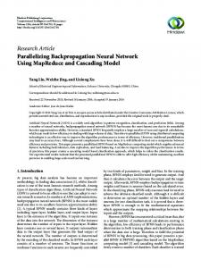
It is known that neural networks interpolate well within the input space, and therefore the network is expected to reproduce the dataset that was used to train it with relatively good accuracy (McKinnell, 2002; Habarulema et al., 2007). Since the main aim is to compare the performance accuracies of the training algorithms on the training dataset, part of the training dataset can still be used in the final verification of the models. This can be referred to as the determination of the correct application of the neural network technique on a particular dataset. The overall verification of the models was performed using Sutherland (2003 and 2008) and Cape Town (2002) datasets. While it is expected that the network should perform very well for SUTH 2003 data (part of the training dataset), the differences between algorithm performances should be evident if present. Figure 1 shows the scatter plot for hourly GPS TEC and modelled TEC values using different NN training algorithms over SUTH for 2003. Correlation coefficient values indicate a slightly better performance by the L-MBP algorithm compared to the rest of the considered algorithms. The widely used algorithms (SBP and L-MBP) in ionospheric modelling provide improved interpolation of TEC estimates. Although the model was tested on the “seen” dataset (2003), it was noted that all training algorithms achieved over 90 % accuracy (over the entire dataset, denoted as “all hours” in Table 2) in estimating TEC, and their modelling results are highly comparable. Ann. Geophys., 30, 857–866, 2012

y=0.935x+0.3567 R=0.9229

20 30 40 BPB TEC (TECU)

70 60 y=0.9778x−0.2034 50 R=0.9309 40 30 20 10 0 0 10 20 30 40 BPM TEC (TECU) 70 60 50 y=0.9676x−0.6565 40 R=0.9312 30 20 10 0 0 10 20 30 40 SBP TEC (TECU)

50

60

GPS TEC (TECU)

10

50

60

GPS TEC (TECU)

GPS TEC (TECU) GPS TEC (TECU)

70 60 50 40 30 20 10 0 0

GPS TEC (TECU)


GPS TEC (TECU)

860

50

60

70 60 y=0.973x−0.405 50 40 R=0.9303 30 20 10 0 0 10 20 30 40 BPC TEC (TECU) 70 60 y=0.9778x−0.2034 50 R=0.9309 40 30 20 10 0 0 10 20 30 40 BPWD TEC (TECU) 70 60 50 40 30 20 10 0 0

50

60

50

60

50

60

y=0.9638x−0.0285 R=0.9381

10

20

30

40

L−MBP TEC (TECU)

Fig. 1. Scatter plots for hourly GPS TEC and corresponding modelled TEC values using different NN training algorithms for Sutherland in 2003.

Table 3. Computed correlation coefficient values for CPTN in 2002. Training

Correlation coefficients at different times (UT)

algorithm

all hours

04:00

10:00

16:00

22:00

BPB BPC BPM BPWD SBP L-MBP

0.9514 0.9589 0.9585 0.9585 0.9589 0.9563

0.7705 0.7733 0.7785 0.7785 0.7768 0.7896

0.8705 0.8885 0.8840 0.8841 0.8887 0.8785

0.8804 0.8925 0.8951 0.8951 0.8943 0.8744

0.7475 0.7866 0.7900 0.7900 0.7883 0.8067

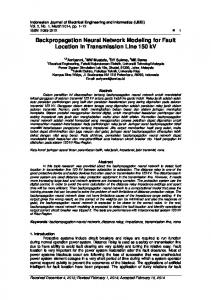
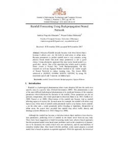
Figure 2 shows the computed RMSE values between GPS TEC and modelled TEC using the six algorithms considered at local sunrise (04:00 UT), midday (10:00 UT), sunset (16:00 UT) and midnight (22:00 UT) over SUTH in 2003. Superimposed on these plots is the GPS TEC variability at these respective times. Table 2 is a summary of the correlation coefficients computed using GPS derived TEC and modelled TEC (from 6 algorithms) for hourly data, 04:00 UT, 10:00 UT, 16:00 UT and 22:00 UT over SUTH in 2003. For Ann. Geophys., 30, 857–866, 2012

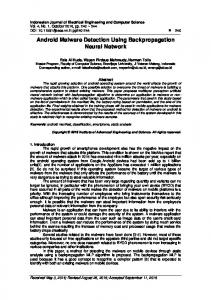
the “seen” data, it was observed that the L-MBP algorithm performs well for local sunrise and midday TEC estimates. Figure 3 shows the scatter plot for GPS TEC and modelled TEC for the “unseen” data over CPTN in 2002. Table 3 shows the corresponding correlation coefficients for local sunrise, midday, sunset and midnight hours. RMSE values for similar periods are graphically shown in Fig. 4 with superimposed GPS TEC values. The following summarises the observations made from Table 3 and Figs. 3 and 4: – In terms of correlation coefficients, all algorithms achieved over 95 % prediction accuracy. However, to draw a conclusion on the overall performance of any algorithm, more than one statistical technique is required. An example is the SBP algorithm, which gives a correlation coefficient value for 16:00 UT that is less than those for BPM and BPWD algorithms (Table 3), but gives the least RMSE value for 16:00 UT (see Fig. 4). – During periods of low TEC variability (04:00 UT and 22:00 UT) the accuracy of all algorithms reduce. Although it is assumed that the ionospheric shell height is 350 km in the derivation of TEC data, which were later www.ann-geophys.net/30/857/2012/


120

180

240

300

360 30

60

120

25

04h00 UT RMSE (TECU)

0

8

3.5

20 15

3

10 2.5

180

240

300

360 70 60

10h00 UT

7.5

50 40

7

30 20

6.5

5 2

BPB BPC BPM BPWD SBP L−MBP

10

0

6


Training algorithm

6

60

Day number (2003) 120 180 240 300

Training algorithm Day number (2003) 360 60

3

50

2.8

RMSE (TECU)

16h00 UT 5.5

40 30

5

20 4.5

10 4


0

0

60

120

180

240

300

360 20

22h00 UT GPS TEC (TECU) RMSE (TECU)

0

0

15

2.6

10 2.4

5

2.2 2

Training algorithm


GPS TEC (TECU)

60

GPS TEC (TECU) RMSE (TECU)

0

4

Day number (2003)

GPS TEC (TECU)

Day number (2003)

861

0

Training algorithm

Fig. 2. GPS TEC values and RMSE values computed for modelled TEC using different algorithms at 04:00 UT, 10:00 UT, 16:00 UT and 22:00 UT, respectively, over SUTH 2003.

used in models development as target values, in reality the shell height varies with time and solar activity levels. Given that 350 km is the typical day-time ionospheric shell height in mid-latitude regions, the reduction in algorithm prediction accuracy during low TEC variability periods could be related to the assumption of a constant value. During nighttime (in absence of ionisation) the shell height increases. – At local midday and sunset the SBP algorithm gives improved TEC estimates compared to other algorithms. – Algorithms BPM and BPWD almost have the same accuracy. Their difference (where it exists) in prediction performance is significantly small (∼ 1 × 10−4 and (1 − 3) × 10−4 TECU for correlation coefficient and RMSE, respectively). For any specific time selected, the performance differences of all the algorithms are not significantly large (as quantified by correlation coefficient and RMSE values), apart from results shown in Fig. 2 where the L-MBP algorithm interpolates exwww.ann-geophys.net/30/857/2012/

ceptionally well at 04:00 UT over SUTH. What is quite distinct is that the performance of all algorithms on “seen” data (SUTH 2003) is lower than their corresponding performance on “unseen” data (CPTN 2002). Figure 5 shows the GPS TEC data that was used for the model development, along with daily sunspot numbers to also demonstrate the correlation between solar activity and ionospheric TEC behaviour. This figure reveals that there was missing data for 2001 and almost half of 2004. The years 2003 and 2004 were in the declining phase of the sunspot cycle, and the absence of 2004 data could have contributed to the observed low prediction accuracies of the NN algorithms for the “seen” data. 4.2

Extrapolation results

Daily TEC values for January, February and March 2008 were modelled using NN models developed with the SUTH 2000–2007 dataset. This was done to assess the generalisation capability of the investigated algorithms in extrapolation Ann. Geophys., 30, 857–866, 2012

GPS TEC (TECU)

120 y=1.045x−1.2919 100 R=0.9589 80 60 40 20 0 0 10 20 30 40 50 60 70 80 90 SBP TEC (TECU)

GPS TEC (TECU)

120 100 y=1.0682x−0.9482 R=0.9585 80 60 40 20 0 0 10 20 30 40 50 60 70 80 90 BPM TEC (TECU)

120 y=1.0541x−1.086 100 R=0.9589 80 60 40 20 0 0 10 20 30 40 50 60 70 80 90 BPC TEC (TECU) 120 y=1.0682x−0.9482 100 R=0.9585 80 60 40 20 0 0 10 20 30 40 50 60 70 80 90 BPWD TEC (TECU)

GPS TEC (TECU)

GPS TEC (TECU)

120 100 y=1.0912x−2.3186 R=0.9514 80 60 40 20 0 0 10 20 30 40 50 60 70 80 90 BPB TEC (TECU)

GPS TEC (TECU)


GPS TEC (TECU)

862

120 y=1.0485x−1.0194 100 R=0.9563 80 60 40 20 0 0 10 20 30 40 50 60 70 80 90 L−MBP TEC (TECU)

Fig. 3. Similar to Fig. 1, but for Cape Town in 2002.

of TEC data outside the temporal range used in developing the models. Figure 6 shows average diurnal TEC variations for January, February and March 2008 over SUTH. While the variability of TEC values generated by the L-MBP algorithm can be seen to be far from other values (for January and February 2008), the prediction performances cannot be easily infered from this figure. Computed RMSE values between derived GPS TEC and modelled TEC are shown in Fig. 7. Generally, BPC, BPM, BPWD and SBP algorithms are consistent in their performances for the three months. Presented extrapolation results show that BPM and BPWD provide better TEC estimates with L-MBP giving the least accuracy for January 2008. This is also reflected in Table 4, which shows the RMSE values between GPS TEC and modelled TEC data for the first 10 days in January 2008. Statistically, average values indicate better performance for BPM and BPWD algorithms. There are observed fluctutations in performance levels for different algorithms. BPC and SBP have almost the same performance for February 2008, while L-MBP gives better TEC estimates for March 2008. At this stage our results are therefore inconclusive about the preferred algorithm for exAnn. Geophys., 30, 857–866, 2012

Table 4. Computed RMSE values for the first 10 days in January 2008 over SUTH. Day Jan 08

RMSE (TECU) between GPS and modelled TEC BPB

BPC

BPM

BPWD

SBP

L-MBP

1 2 3 5 6 7 8 9 10

2.8333 1.6280 1.2564 5.4457 2.6385 2.1040 1.7925 2.0558 1.8872

2.7272 1.1237 1.2260 5.4742 2.4754 1.8599 1.7212 1.9382 1.3677

2.8009 1.2628 1.3285 5.7203 2.2284 1.5909 1.6681 1.7954 1.2846

2.8006 1.2630 1.3284 5.7201 2.2285 1.5911 1.6680 1.7955 1.2848

2.7218 1.1797 1.2177 5.4579 2.4856 1.8826 1.6345 1.9409 1.4350

2.2781 1.7804 1.6202 4.6063 2.9358 3.0268 2.8511 3.4634 2.4774

Ave.

2.4046

2.2126

2.1866

2.1867

2.2173

2.7822

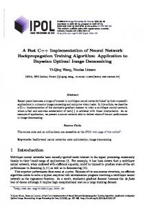
trapolating improved TEC data. From Table 4, it is observed that RMSE values for 5 January 2008 are higher than the other days’ values. Figure 8 shows diurnal TEC variability for 3–6 January 2008, along with Dst and Kp indices. Superimposed on the GPS TEC plot are the modelled TEC values www.ann-geophys.net/30/857/2012/


120

180

240

Day number (2002) 300

360

0 10

30

60

120

5

15 10

4.5

300

360 80

9.5 RMSE (TECU)

RMSE (TECU)

20

GPS TEC (TECU)

04h00 UT

240

10h00 UT

25 5.5

180

60 9

40

8.5

20

5 4

BPB

0

BPC BPM BPWD SBP L−MBP Training algorithm

8

BPB

Day number (2002) 0

9

60

120

180

240

Day number (2002) 300

360

80

5

60

4.5

0

60

16h00 UT

120

180

240

300

40

7.5

20

RMSE (TECU)

8

GPS TEC (TECU)

22h00 UT

8.5

RMSE (TECU)

0


360

30 25 20

4

15 10

3.5

GPS TEC (TECU)

60

GPS TEC (TECU)

Day number (2002) 0 6

863

5 7

BPB

BPC

0

BPM BPWD SBP L−MBP

3

Training algorithm

BPB


0

Fig. 4. Similar to Fig. 2, but for CPTN 2002.

110 240 220

90

200

80

180

70

160

60

140 120

50

100

40

Sunspot number

TEC (TECU)

100

80 30

60

20

40

10 0

20 2000

2001

2002 2003 2004 Time (2000−2007)

2005

2006

2007

0

Fig. 5. Hourly GPS TEC data over SUTH (2000–2007) used for NN training along with daily sunspot number.

generated by the L-MBP algorithm, which gives the smallest RMSE value for 5 January 2008. The Kp index had a constant value of 3.7 from ∼06:00–14:00 UT with Dst varying in the range of 15 to −18 nT. During this period, the AE index (not shown) reached a maximum value of 619 nT www.ann-geophys.net/30/857/2012/

from 60 nT, and remained highly variable even on the next day when TEC showed an irregular and declining trend. The next high Kp index observed is 4 when the Dst index was −26 nT at 23:00 UT. A magnetic substorm occurred on 5 January 2008 (Xu-Dong et al., 2010), which could have caused an increase in TEC compared to the previous 3 January 2008 TEC values. Maximum TEC of ∼27 TECU is observed at 12:00 UT on 5 January 2008 in contrast to a maximum value of ∼20 TECU at 10:00 UT on 3 January 2008. Additionally, the foF2 value over Grahamstown (33.30◦ S, 26.53◦ E), South Africa, increased from 5.5 MHz on 4 January 2008 to 7.325 MHz on 5 January 2008 at 12:00 UT, and later reaching a maximum value of 7.725 MHz at 12:45 UT. This is a difference of 1.825 MHz for 4–5 January 2008 compared to 0.625 MHz for 3–4 January 2008 at 12:00 UT. An investigation of storm time TEC variability over South Africa during a geomagnetic storm of 15 May 2005 reported TEC enhancement and attributed it to the travelling ionospheric disturbances (Ngwira et al., 2012). It appears that substorm activity may also lead to TEC enhancement at South African midlatitude stations; however, a specific mechanism responsible for the observed event in this paper has not been investigated yet.

Ann. Geophys., 30, 857–866, 2012

864

J. B. Habarulema and L.-A. McKinnell: Backpropagation training algorithms in TEC estimations 20

(a)

15

January 2008

10 5 BPB

Modelled or GPS TEC (TECU)

0

BPC

BPM

BPWD

SBP

L−MBP

GPS

(b)

15 10

February 2008

5 0

(c)

15 10

March 2008

5 0 0

2

4

6

8

10

12 Time (UT)

14

16

18

20

22

24

Fig. 6. Hourly average modelled and GPS TEC values for January, February and March 2008 over SUTH.

3 30

2

TEC (TECU)

January 2008

1

20

03 Jan 2008

04 Jan 2008

05 Jan 2008

06 Jan 2008

GPS TEC L−MBP TEC

10 0

February 2008

2 1

Kp

0 3 March 2008

2 1 0

BPB

BPC

BPM BPWD Training algorithm

SBP

L−MBP

9 8 7 6 5 4 3 2 1 0

4 8 12 16 20 0 4 8 12 16 20 0 4 8 12 16 20 0 4 8 12 16 20 0 40 30 20 10 0 −10 −20 −30 4 8 12 16 20 0 4 8 12 16 20 0 4 8 12 16 20 0 4 8 12 16 20 0 Time (UT)

Dst (nT)

RMSE (TECU)

0 3

Fig. 8. Diurnal TEC values for 3–6 January 2008. Dst and Kp indices for this period are also shown.

Fig. 7. RMSE values for January, February and March 2008.

5

Conclusions

This paper has presented results comparing performance levels of some backpropagation algorithms for ionospheric TEC estimations. Similar to other sources (e.g. Jang et al., 1997; Ann. Geophys., 30, 857–866, 2012

Yilmaz et al., 2009), it is evident that the L-MBP algorithm requires the fewest number of iterations, compared to other algorithms, to achieve generalisation. The reported convergence time (∼3 min) is expected to reduce with improved computing capacity. For TEC modelling, the differences in accuracy between the investigated algorithms is not very significant. What is worth noting, though, is the time it takes www.ann-geophys.net/30/857/2012/

J. B. Habarulema and L.-A. McKinnell: Backpropagation training algorithms in TEC estimations each algorithm to achieve convergence or generalisation. This time can increase or decrease depending on the size of the dataset under consideration. This investigation was conducted using a dataset of ∼50 300 data points. Each algorithm can generally be used depending on user requirements and available resources. For small datasets, the MatLab based L-MBP algorithm is sufficient. With more computing power, the other training algorithms can be used to slightly improve the accuracy. BPM and BPWD algorithms appear to achieve the same accuracy in a relatively short period of time and may be advantageous over the SBP algorithm, which has been widely used for modelling various ionospheric parameters. According to Zell et al. (1998), the momentum term (in the BPM) leads to the computation of the new weight change using the old weight change (during training), thereby mimimising oscillations associated with SBP for narrow minimum area error surfaces. BPM is a simple modification of SBP which accelerates the training/learning process (Rojas, 1996), and this is clearly evident in Table 1 in terms of the time and number of epochs required to achieve convergence.

Acknowledgements. J. B. Habarulema’s research is supported by the South African National Space Agency (SANSA) and National Research Foundation (NRF), South Africa. The GPS data was provided by the Chief Directorate: National Geo-spatial information, South Africa. Topical Editor K. Kauristie thanks two anonymous referees for their help in evaluating this paper.

References Cander, L. R.: Artificial neural network applications in ionospheric studies, Annali De Geofisica, 5–6, 757–766, 1998. Cander, L. R., Milosavljevic, M. M., Stankovic, S. S., and Tomasevic, S.: Ionospheric forecasting technique by artificial neural network, Electronic letters, 34, 1573–1574, 1998. Chan, A. H. Y. and Cannon, P. S.: Nonlinear forecasts of foF2: variation of model predictive accuracy over time, Ann. Geophys., 20, 1031–1038, doi:10.5194/angeo-20-1031-2002, 2002. Demuth, H., Beale, M., and Hagan, M.: Neural Networkbox Box™ 6 User’s Guide, The MathWorks™ , 2009. Habarulema, J. B., McKinnell, L. A., and Cilliers, P. J.: Prediction of global positioning system total electron content using neural networks over South Africa, J. Atmos Solar Terr. Phys., 69, 1842–1850, 2007. Habarulema, J. B., McKinnell, L.-A., and Opperman, B. D. L.: A recurrent neural network approach to quantitatively studying solar wind effects on TEC derived from GPS; preliminary results, Ann. Geophys., 27, 2111–2125, doi:10.5194/angeo-272111-2009, 2009. Habarulema, J. B., McKinnell, L.-A., and Opperman, B. D. L.: TEC measurements and modelling over Southern Africa during magnetic storms; a comparative analysis, J. Atmos. Solar Terr. Phys., 72, 509–520, 2010. Haykin, S.: Neural Networks, A Comprehensive Foundation, Macmillan College Publishing Company, 1994.

www.ann-geophys.net/30/857/2012/

865

Heilig, B., Lotz, S., Verõ, J., Sutcliffe, P., Reda, J., Pajunpäa¨ , K., and Raita, T.: Empirically modelled Pc3 activity based on solar wind parameters, Ann. Geophys., 28, 1703–1722, doi:10.5194/angeo28-1703-2010, 2010. Hernàndez-Pajares, M., Juan, J., and Sanz, J.: Neural network modelling of the ionospheric electron content at global scale using GPS, Radio Sci., 32, 1081–1090, 1997. Jang, J. S. R., Sun, C. T., and Mizutani, E.: Neuro Fuzzy and Soft Computing, Prentice-Hall, Upper Saddle River, New Jersey, 1997. Leandro, R. F. and Santos, M. C.: A neural network approach for regional vertical total electron content modelling, Studia Geophysica et Geodaetica, 51, 279–292, 2007. Lundestedt, H.: Solar activity modelled and forecasted: A new approach, Adv. Space Res., 38, 862–867, 2006. Lundstedt, H., Gleisner, and Wintoft, P.: Operational forecasts of the geomagnetic Dst index, Geophys. Res. Lett., 29, 2181, doi:10.1029/2002GL016151, 2002. McKinnell, L.-A.: A Neural Network based Ionospheric model for the bottomside electron density profile over Grahamstown, South Africa, Ph.D. thesis of Rhodes University, Grahamstown, South Africa, 2002. McKinnell, L.-A. and Poole, A. W. V.: Predicting the ionospheric F layer using neural networks, J. Geophys. Res., 109, A08308, doi:10.1029/2004JA010445, 2004. Ngwira, C. M., McKinnell, L.-A., Cilliers, P. J., and Yizengaw, E.: An investigation of ionospheric disturbances over South Africa during the magnetic storm on 15 May 2005, Adv. Space Res., 49, 327–335, 2012. Opperman, B.: Reconstructing Ionospheric TEC over South Africa using signals from a Regional GPS network, PhD thesis Rhodes University, Grahamstown, South Africa, 2007. Opperman, B. D. L., Cilliers, P. J., McKinnell, L. A., and Haggard, R.: Development of a regional GPS-based ionospheric TEC model for South Africa, Adv. Space Res., 39, 808–815, 2007. Oyeyemi, E. O., McKinnell, L.-A., and Poole, A. W. V.: Nearreal time foF2 predictions using neural networks, J. Atmos. and Solar-Terr. Phys., 68, 1807–1818, 2006. Reczko, M., Riedmiller, M., Seemann, M., Ritt, M., DeCoster, J., Biedermann, J., Danz, J., Wehrfritz, C., Werner, R., Berthold, M., and Orsier, B.: External contributions to Stuttgart Neural Network Simulator (SNNS), User Manual, Version 4.2, Universities of Stuttgart and Tübingen, Germany, and the European Particle Research Lab, CERN, Geneva, Switzerland, 1998. Rojas, R.: Neural Networks – A Systematic Introduction, SpringerVerlag, Berlin, Germany, New-York, USA, 1996. Schaer, S.: Mapping and Predicting the Earth’s Ionosphere Using the Global Positioning System, Ph.D. thesis, Astronomical Institute, University of Berne, Berne Switzerland, 1999. Senalp, E. T., Tulunay, E., and Tulunay, Y.: Total electron content (TEC) forecasting by Cascade Modeling, A possible alternative to the IRI-2001, Radio Sci., 43, RS4016, doi:10.1029/2007RS003719, 2008. Tulunay, E., Senalp, E. T., Cander, L. R., Tulunay, Y. K., Bilge, A. H., Mizrahi, E., Kouris, S. S., and Jakowski, N.: Development of algorithms and software for forecasting, nowcasting and variability of TEC, Ann. Geophys., 47, 1201–1214, 2004. Tulunay, E., Senalp, E., Radicella, S., and Tulunay, Y.: Forecasting total electron content maps by neural network technique, Radio

Ann. Geophys., 30, 857–866, 2012

866


Sci., 41, RS4016, doi:10.1029/2005RS003285, 2006. Vandegriff, J., Wagstaff, K., and G. Ho, J. P.: Forecasting space weather: Predicting interplanetary shocks using neural networks, Adv. Space Res., 36, 2323–2327, 2005. Weigel, R. S., Vassiliadis, D., and Klimas, A. J.: Coupling of the solar wind to temporal fluctuations in ground magnetic fields, Geophys. Res. Lett., 29, 1915, doi:10.1029/2002GL014740, 2002. Weigel, R. S., Klimas, A. J., and Vassiliadis, D.: Solar wind coupling to and predictability of ground magnetic fields and their time derivatives, J. Geophys. Res., 108, 1298, doi:10.1029/2002JA009627, 2003. Xu-Dong, Z., Ai-Min, D., Wen-Yao, X., Yuan, W., and Hao, L.: A near Earth reconnection of the magnetospheric substorm on January 5, 2008: THEMIS observations, Chinese J. Geophys., 53, 1019–1027, 2010.

Ann. Geophys., 30, 857–866, 2012

Yilmaz, A., Akdogan, K. E., and Gurun, M.: Regional TEC mapping using neural networks, Radio Sci., 44, RS3007, doi:10.1029/2008RS004049, 2009. Zell, A., Mamier, G. M., Vogt, M., Mache, N., Hübner, R., Döring, S., Herrmann, K.-U., Soyez, T., Schmalzl, M., Sommer, T., Hatzigeorgiou, A., Posselt, D., Schreiner, T., Kett, B., Clemente, G., Wieland, J., and Gatter, J.: Stuttgart Neural Network Simulator (SNNS), User Manual, Version 4.2, Universities of Stuttgart and Tübingen, Germany, and the European Particle Research Lab, CERN, Geneva, Switzerland, 1998.

www.ann-geophys.net/30/857/2012/