NESUG 16
Statistics, Data Analysis & Econometrics
st008
A Backwards-Manual Selection Macro for Binary Logistic Regression in the SAS® v.8.02 PROC LOGISTIC Procedure. Janice Hegewald, Annette Pfahlberg, and Wolfgang Uter, Institute of Medical Informatics, Biometry, and Epidemiology, Erlangen, Germany ABSTRACT Multivariate logistic regression is often used within the field of epidemiology to describe the relationship between disease occurrence and an exposure suspected to be associated with the disease. Additional effects are added to the model if they confound the disease-exposure relationship. Traditional model selection procedures, which focus on selecting models that are good predictors of the dependent variables, are not necessarily the most appropriate for epidemiological research questions. The proposed backwards-manual selection macro, %bms, attempts to select logistic regression models more suitable for epidemiological research. The macro consists of two main stages, (1) backwards selection of effect-modifiers, and (2) selection of main effects based on their confounding potential and influence on overall model-fit. During the first stage, the macro generates all first-order effect modifiers for the variables provided by the user, and PROC LOGISTIC’s backwards selection option is used to remove non-significant effect-modifiers. The second stage begins by removing the least significant potential confounder from the model. If this does not cause a change in the relationship between disease and exposure or the overall model fit, it remains out of the model. This process continues until all of the potential confounders not included in an effect-modifier have been evaluated. Keywords: logistic regression, PROC LOGISTIC, model selection, epidemiology, Odds Ratio
BACKGROUND Selecting the proper logistic regression model is a critical and often difficult initial step in the analysis of data with the multivariate logistic regression. While the selection of effects to be included in a logistic regression model can be quickly and conveniently conducted in SAS ® v. 8.02 (Cary, NC) with the selection options built into PROC LOGISTIC, the resulting models may not be the most appropriate or valid for addressing certain research questions. These selection methods select or exclude model effects according to the amount of dependent variable variation that they explain. While the objective of these selection methods is consistent with the general principle of logistic regression, the resulting models may not be suitable for logistic
regression models designed to examine one independent variable while controlling for the effects of other independent variables. The models resulting from conventional selection procedures may contain superfluous variables that are unnecessary to address the research question at hand and lack variables that are important due to their effect modification or confounding properties, but alone do not significantly improve the model’s prediction of the dependent variable values. Multivariate logistic regression is widely used in health research, because it facilitates the analysis of the relationship between a binomial dependent variable, such as the occurrence of disease (D) and a single independent variable, or exposure (E). One of the most appealing features of multivariate logistic regression is that causal confounders, variables that may obfuscate the relationship of interest, can be entered into the model and held constant. This permits a controlled examination of the relationship between D and E. Selecting valid models for healthrelated research requires careful deliberation, a thorough examination of potential confounders and their effects on the relationship of interest, as well as consideration of the biological or social mechanisms that are the underlying basis for the confounding. Some researchers favor the inclusion of all potential confounders in a model to ensure that all possible confounding is controlled, however, this may not be a viable solution if there are many potential confounders. Health research studies are often limited in size due to financial, ethical, or biological constraints, and regression models with many effects, or more specifically a large effect- tosample-size ratio may be unstable and result in increased estimated standard errors. [Hosmer, 1989] Algorithms for identifying or selecting confounders for epidemiological research have been proposed for both stratified and regression analyses [Kleinbaum, 1982; Rothman, 1998, Greenland, 1989]. These procedures often involve some form of change-inestimate (CE) assessment [Greenland, 1989]. CE selection procedures select confounding variables according to the amount of change in the estimate of E observed as variables are added or removed from a regression model or stratified analysis. These methods are more involved than those available with PROC LOGISTIC, and lack readily available software packages.
NESUG 16
Statistics, Data Analysis & Econometrics
Kleinbaum, Kupper and Morgenstein [1982] proposed a selection procedure specifically for logistic regression, which involves the examination of effect modifiers, followed by the examination of changes to the Odds Ratios (OR) for E with various subsets of the remaining potential confounders. A subset of variables is selected when they produced a noticeable change to the OR. Finally, additional effects were entered into the model if they improved the precision of the estimated OR.
When the %bms macro is run it begins by calling the %varsin sub-macro. %varsin writes the independent variables (&E, &C1, &C2) into the temporary dataset work._variables. As variables are r emoved from the model they are deleted from the work._variables dataset.
Table 1: %bms Macro variables
The Backwards-Manual Selection (BMS) algorithm and corresponding macro follows portions of the general variable assessment sequence proposed by Kleinbaum, Kupper, and Morgenstein in their modeling algorithm, and is in effect an automation of a “manual” evaluation of potential confounders. First, BMS eliminates effect modifiers from the binomial logistic regression models based on their significance level. Secondly, main effects of potential confounders are selected for elimination if they do not influence the estimated OR of the independent variable of interest and have a negative influence on the global model-fit.
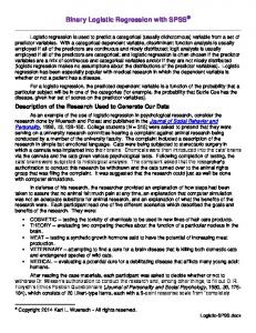
METHODS The %bms macro was created and tested with SAS to perform the backward manual selection algorithm for selecting multivariate binomial logistic regression models. The macro consists of three sub-macros, %varsin, %effmod and %confound, which prepare the variables for the selection procedure, evaulate effect modification, and assess confounding and global model fit, respectively. A flowchart of the %bms macro can be found in Figure 1. Upon initiation of the macro, several macro variables must be defined (Table 1). These macro variables correspond to the model variables and control optional settings incorporated into the macro. The binomial dependent variable should be listed as D, and the main independent of interest should be listed as E. Well documented confounders or confounders chosen a priori can be listed as C1 (separated by a space). C1 variables are be included in every run of PROC LOGISTIC and are not be evaluated for confounding. Potential confounders that are to be analyzed by the %bms should be listed as C2. Any categorical C1 or C2 variables should also be listed in the macro variable ‘CLASS’, and not entered into %bms as dummy variables. This facilitates the assessment of their combined influence on the D-E relationship. The macro variables p, k, and g define significance levels and the amount of change to detect during certain stages of the selection procedure. The macro variable EM controls the running of the sub-macro %effmod, and the subsequent evaluation of effect modification. and TEST selects the global model fit test to be used.
If the macro option EM has been selected (EM=yes), then the %bms macro will call the optional %effmod sub-macro after the completion of the %varsin submacro. %effmod creates all of the possible effect modifiers and runs PROC LOGISTIC with the built-in backwards selection option set to remove only the newly created effect modifiers from the model if they do not meet the user-defined significance level 2 (Wald X statistic) [SAS 1999]. If the user does not list a value for p, the macro will use the default value of p=0.10. Note: this is not the SAS default p-value for the PROC LOGISTIC backward selection option. At the conclusion of %effmod, the hierarchal rule is applied so that main effects included in the remaining effect modifiers will not be analyzed or deleted during processing of the %confound macro. The third and last sub-macro, %confound, evaluates the effect of removing a potential confounder from the model on the OR of the E variable. Each potential confounder that was not determined to be an effect modifier is assessed individually in order of ascending significance (descending p-value). In other words, the least significant potential confounder is considered for removal from the model first. If removing a potential confounder (C2) results in the proportion of the absolute difference in the two OR estimates divided by the OR from the model with the potential confounder to be more than k (default k =0.10), then the variable is considered a confounder and remains in the model,. k < |ORwithC2 – ORwithoutC2| / ORwithC2.
(1)
NESUG 16
Statistics, Data Analysis & Econometrics
Fig. 1 Flowchart of the %bms Macro
Variables not causing a large enough difference in the OR of E to be kept in the model are considered to have no substantial confounding effect. However, it may be advantageous to keep a ‘non-confounder’ in the model when if it greatly improves the model’s overall fit. Therefore, a second exclusion criteria for global fit-tests can also be implemented. If the TEST macro variable has been defined as Pearson or HL, raw differences to the Pearson or HosmerLemeshow goodness-of-fit-tests p-values are evaluated, respectively. Variables that appear to have a strong positive effect on the model fit p-value (raw difference +0.20) are not excluded from the model, even if they had no confounding potential. Non-confounders with little or negative influence on
the goodness-of-fit are removed from the model. If the results from either of the global fit tests prove to be unsuitable for the dataset, the goodness-of-fit evaluation can be omitted by defining it with a blank space (TEST= ). At the conclusion of the %confound macro all temporary datasets generated by the macro are deleted, a summary of the selection process and a list of the independent variables of the proposed final model are printed to the OUTPUT window, and PROC LOGISTIC is run one last time with the effects of the final model. Details of the %bms procedures, i.e. the generation of effect modifiers, calculation of the change in OR, etc. are written to the log.
NESUG 16
Statistics, Data Analysis & Econometrics
LIMITATION OF USE One of the strengths of logistic regression and PROC LOGISTIC, is flexibility. Unfortunately, at the moment the %bms macro is unable to handle all of the many possibilities available with logistic regression. At the moment, the %BMS macro requires that the independent variable of interest be binomial, continuous, or ordinal. If the independent variable of interest is nominal with more than two categories, then program can only assess one of the variable levels. This assessment will not be representative of the overall change in the E variable.
LOW BIRTHWEIGHT EXAMPLE Data on low birth weight risk factors used by Hosmer and Lemeshow in Applied Logistic Regression to demonstrate model selection were used to demonstrate the %bms macro and compared with the results of the model selection procedures available with PROC LOGISTIC [Hosmer, 1989]. The response was coded as the occurrence of low birth weight (LOW=1) versus a normal birth weight (LOW=0). For this example the risk factor of interest (E) was defined as smoking during pregnancy (SMOKE). The remainder of the dataset variables are described briefly in Table 2. The %bms selection procedure was called with the following statement:
%bms (D= low , E= smoke, C1=age , C2= lwd race ptd ht ui ftv, CLASS= race, EM=yes, p= ,k= , g= , TEST=HL, DSN= lowbwt) ; AGE was defined as a known confounder (C1) due to its biological and social potential to confound, and the remaining variables, LWD, RACE, PTD, HT, UI, and FTV, were listed as potential confounders (C2). RACE was also defined as a categorical variable in the CLASS statement. To be consistent with Hosmer and Lemeshow’s example, the variables for the mother’s weight at last menstrual period (LWD) and a history of premature labors (PTD) were converted to a binary variables. The macro was set to evaluate effect modification (EM=YES) and the HosmerLemeshow Goodness of Fit Test (TEST=HL). The %effmod sub-macro generated all of the seven possible effect modifiers. All of the effect modifiers were eliminated from the model, because they failed to meet the %bms macro’s default significance level of 0.10. During the running of the %confound sub-macro the removal of the variables RACE and PTD caused a greater than 10% change in the OR for SMOKE, and therefore were not removed from the model. The
Table 2: Low birthweight variables
variables HT and LWD did not have an substantial effect on the OR, but were kept in the model because they improved the results of the Hosmer & Lemeshow goodness-of-fit test more than the default level of 0.20. The variables UI and FTV were removed from the model because they had no appreciable influence on the estimate for SMOKE or the global fit. Forward, Backward and Stepwise selection with PROC LOGISTIC’s default inclusion and exclusion criteria were also conducted with the provision that the independent variables for SMOKE and AGE be included in every model. All three procedures resulted in the same final model (Table 3). While this model is more parsimonious than the resulting %bms model, the variable RACE was not included in the final model. Changes to the estimate of SMOKE suggest that RACE is a causal confounder for this research question. Consequently, the model unadjusted for RACE may not be the best model for a valid interpretation of the exposure variable SMOKE. Table 3: Comparison of final models.
CONCLUSIONS The %bms macro provides an automated alternative to the selection procedures available with PROC LOGISTIC. The model selected by the BMS procedure are likely to be more appropriate where the confounding takes precedence over predictionpotential of the dependent variable values in the selection of variables.
NESUG 16
Statistics, Data Analysis & Econometrics
REFERENCES Greenland, S. (1989). “Modeling and Variable Selection in Epidemiologic Analysis.” Am J of Public Health 79(3): 340-349. Hosmer, D. and S. Lemeshow (1989). Applied Logistic Regression. New York, Wiley. Kleinbaum, D., L. Kupper, et al. (1982). Epidemiological Research, Principles and Quantitative Methods. New York, Wiley. Rothman, K. J. and S. Greenland (1998). Modern Epidemiology. Philadelphia, PA, Lippincott-Raven. SAS Institute Inc. (1999). SAS/STAT(R) User's Guide, Version 8. Cary, NC, SAS Institute Inc.
ACKNOWLEDGEMENTS SAS is a registered trademark of SAS Institute Inc. in the USA and other countries. ® indicates USA registration.
CONTACT INFORMATION The %bms macro is available on-line at http://www.imbe.med.uni-erlangen.de/ issan/ issan.htm or will be provided upon request. Questions or comments should be addressed to: ATTN: Janice Hegewald IMBE, University of Erlangen Waldstr. 6 D-91054 Erlangen Germany Tel.: 49 (9131) 85-25738 Fax: 49 (9131) 85E-mail:
[email protected]