BMC Medical Research Methodology
BioMed Central
Open Access
Research article
Beyond logistic regression: structural equations modelling for binary variables and its application to investigating unobserved confounders Emil Kupek* Address: National Perinatal Epidemiology Unit, Institute of Health Sciences, University of Oxford, UK Email: Emil Kupek* -
[email protected] * Corresponding author
Published: 15 March 2006 BMC Medical Research Methodology2006, 6:13
doi:10.1186/1471-2288-6-13
Received: 16 December 2005 Accepted: 15 March 2006
This article is available from: http://www.biomedcentral.com/1471-2288/6/13 © 2006Kupek; licensee BioMed Central Ltd. This is an Open Access article distributed under the terms of the Creative Commons Attribution License (http://creativecommons.org/licenses/by/2.0), which permits unrestricted use, distribution, and reproduction in any medium, provided the original work is properly cited.
Abstract Background: Structural equation modelling (SEM) has been increasingly used in medical statistics for solving a system of related regression equations. However, a great obstacle for its wider use has been its difficulty in handling categorical variables within the framework of generalised linear models. Methods: A large data set with a known structure among two related outcomes and three independent variables was generated to investigate the use of Yule's transformation of odds ratio (OR) into Q-metric by (OR-1)/(OR+1) to approximate Pearson's correlation coefficients between binary variables whose covariance structure can be further analysed by SEM. Percent of correctly classified events and non-events was compared with the classification obtained by logistic regression. The performance of SEM based on Q-metric was also checked on a small (N = 100) random sample of the data generated and on a real data set. Results: SEM successfully recovered the generated model structure. SEM of real data suggested a significant influence of a latent confounding variable which would have not been detectable by standard logistic regression. SEM classification performance was broadly similar to that of the logistic regression. Conclusion: The analysis of binary data can be greatly enhanced by Yule's transformation of odds ratios into estimated correlation matrix that can be further analysed by SEM. The interpretation of results is aided by expressing them as odds ratios which are the most frequently used measure of effect in medical statistics.
Background Statistical problems that require going beyond standard logistic regression Although logistic regression has become the cornerstone of modelling categorical outcomes in medical statistics, separate regression analysis for each outcome of interest is hardly challenged as a pragmatic approach even in the sit-
uations when the outcomes are naturally related. This is common in process evaluation where the same variable can be an outcome at one point in time and a predictor of another outcome in future. For example, preterm delivery is both an important obstetric outcome and a risk factor for low birthweight, which in turn can adversely affect future health. Sequential nature of these outcomes is not Page 1 of 10 (page number not for citation purposes)
BMC Medical Research Methodology 2006, 6:13
http://www.biomedcentral.com/1471-2288/6/13
d1
d2 b
d1
d2
Y1
Y2
X1
X2
X1
X2
X3
X4
e2
e1
e2
e3
e4
e1
r
F
Y
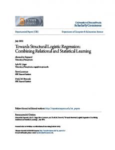
Figure 1 problems needing SEM approach Statistical Statistical problems needing SEM approach.
encompassed by repeated measures models which deal with the same outcome at different time points. Another example of a research problem difficult to handle by logistic regression model is when an outcome is determined not only by direct influences of the predictor variables but also by their unobserved common cause. For example, survival time since the onset of an immune system disease may be adversely affected by concomitant occurrence of various markers of disease progression indicating immunosupression as an underlying common factor, the latter being an unobserved latent variable whose estimation requires solving a system of related regression equations. Structural equation modelling (SEM) is a very general statistical framework for dealing with above issues. In recent years, it has been increasingly used in medical statistics. In addition to traditional areas such as psychometric properties of health questionnaires and tests, behavioural genetics [1], measurement errors [2] and covariance structure in mixed regression models [3] have received particular attention. In addition to specific applications, important research methodology issues in SEM have been given more space in medical statistics, among which a comparison with multiple regression [4], the relevance of latent variable means in clinical trials [5] and power of statistical tests [6] deserve special attention. However, a great obstacle for wider use of SEM has been its difficulty in handling categorical variables. The aim of this paper is to briefly review main aspects of this difficulty and to demonstrate a new approach to this problem based on a simple transformation. Two examples with both simulated and real data are provided to illustrate this approach. SEM includes both observed and unobserved (latent) variables such as common factors and measurement errors. The Linear Structural Relationships (LISREL) model [7]
was the first to spread in psychometric applications due to the availability of software. Other formulations of SEM and corresponding software emerged (see [8] for an overview). The details of these models, as well as important issues regarding their identifiability, estimation and robustness, are beyond the scope of this work but an illustration of the situations where SEM is needed is presented instead (Figure 1). As a general rule, SEM is indicated when more than one regression equation is necessary for statistical modelling of the phenomena under investigation. The left part of Figure 1 shows a situation where two outcomes, denoted Y1 and Y2, are mutually related (a feedback loop) and influenced by two predictors, denoted X1 and X2. For example, the outcomes could be demand and supply of a particular health service or risk perception and incidence of a particular health problem. The predictor variables' error terms, denoted e1 and e2, may be correlated (r) if an important variable influencing both predictors is omitted, i.e. in the case of bias in exposure measures. The terms d1 and d2 indicate disturbances of the two outcomes. The right part of Figure 1 illustrates a combination of common factors and regression model. In this case, it is of interest to test whether the outcome Y is determined not only by direct influences of the predictor variables, denoted X1, X2, X3 and X4, but also by their latent determinant as indicated by the regression coefficient b. SEM has received many criticisms, most of which have been concerned with vulnerability of complex models relying on many assumptions, as well as with uncritical use and interpretation of SEM. These are well placed concerns but are not intrinsic to SEM; even well known and widely applied techniques such as regression share the same concerns. Complex phenomena require complex models whose inferential aspects are more prone to error as the number of parameters increases. SEM is often the only statistical framework by which many of these issues can be addressed by testing and comparing the models obtained [9]. Handling categorical variables in SEM Specific criticism regarding the treatment of categorical and ordinal variables in SEM has been a strong deterrent for its wider use. Naive treatment of binary and ordered categorical variables as if they were normally distributed in some SEM applications was partly due to the lack of viable alternatives in its early days. Inadequate use of standardized regression coefficients as the measures of effect in some SEM applications was also criticised [10]. Even when distributional properties of categorical variables were taken into account, the interpretation of SEM parameter estimates in terms of impact measures such as attributable risk was not applied. Standard errors and
Page 2 of 10 (page number not for citation purposes)
BMC Medical Research Methodology 2006, 6:13
http://www.biomedcentral.com/1471-2288/6/13
Table 1: Simulated data: Observed odds ratios (OR), associated 95% confidence intervals (CI) and SEM regression coefficients with corresponding standard errors (SE) obtained via ML estimation (N = 5000)
Observed association Parameter*
a1 (BIN1→YBIN) a2 (BIN2→YBIN) a3 (BIN3→YBIN) a4 (MBIN→YBIN) b1 (BIN1→MBIN) b2 (BIN2→MBIN) b3 (BIN3→MBIN)
SEM-predicted effects
OR (95% CI) for the variable pairs
Correlation (Q) estimate
Regression estimate (SE) in Q-metric
Regression estimate (95% CI) in OR-metric**
2.138 (1.887, 2.423) 3.711 (3.255, 4.232) 0.364 (0.321, 0.414) 10.883 (9.411, 12.586) 2.632 (2.304, 3.006) 4.095 (3.561, 4.709) 1.083 (0.955, 1.229)
0.3627 0.5755 -0.4660 0.8137 0.4493 0.6075 0.0398
0.0281 (0.0039) 0.1036 (0.0044) -0.4979 (0.0033) 0.7760 (0.0050) 0.4479 (0.0093) 0.6070 (0.0093) 0.0276 (0.0093)
1.058 (1.042, 1.074) 1.231 (1.210, 1.253) 0.335 (0.329, 0.341) 7.929 (7.554, 8.337) 2.622 (2.507, 2.746) 4.089 (3.863, 4.337) 1.0568 (1.019, 1.096)
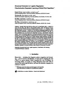
* Arrows point to the dependent variables in the model (see Figure 2) ** Back-transformed from Q to OR by (1+Q)/(1-Q)
confidence limits – rarely used in SEM – are generally underestimating structural model uncertainties such as selection of relevant variables and correct specification of their influences. A recent review of handling categorical and other nonnormal variables in SEM [11] listed four main strategies: a) asymptotic distribution free (ADF) estimators adjusting for non-normality by taking into account kurtosis in joint
d1
d2 a4
MBIN b1
YBIN a3
a1 b2
a2
b3
BIN1
BIN2
BIN3
e1
e2
e3
Figure 2 model Simulated Simulated model.
multivariate distribution [12], b) the use of robust maximum likelihood estimation or resampling techniques such as jacknife or bootstrap to obtain the standard errors of SEM parameters as these are most affected by departure from multivariate normality [13], c) calculating polyserial, tetrachoric or polychoric correlations for pairs of variables with non-normal joint distribution by assuming that these have an underlying (latent) continuous scale whose large sample joint distribution is bivariate normal, then using these correlations as the input for SEM [14], and d) estimating probit or logit model scores for observed categorical variables as the first level, then proceeding with SEM based on these scores as the secondlevel [15]. The ADF estimation generally requires large samples to keep the type II error at a reasonable level and extremely non-normal variables such as binary may be difficult to handle with sufficient precision. The last two strategies critically depend on how well the first-level model fits the data. A review of statistical models for categorical data reveals the lack of a method capable of handling more than one regression equation [16]. Although log-linear models for contingency tables may analyse related categorical outcomes and their relationship with independent variables, possibly complex interactions between the variables in the model do not indicate the direction of influences as in regression models. This underlines the need for a SEM framework for categorical data analysis in order to handle both dimensionality reduction and regression techniques within the same model (cf. the right part of Figure 1). Two major recent developments in handling categorical data include Muthen's extension of SEM to the 'latent variable modeling' approach [17] and an extension of generalized linear models to latent and mixed variables under GLLAMM (Generalized Linear Latent And Mixed Models) framework [18]. Despite coming from different statistical
Page 3 of 10 (page number not for citation purposes)
BMC Medical Research Methodology 2006, 6:13
http://www.biomedcentral.com/1471-2288/6/13
Table 2: Multivariate logistic regression for generated data: parameter estimates (standard errors) for large (N = 5000) and small (N = 100) samples
YBIN outcome
Intercept BIN1 BIN2 BIN3 MBIN
MBIN outcome
N = 5000
N = 100
N = 5000
N = 100
-0.5735 (0.0787) 0.5602 (0.0781) 0.9941 (0.0791) -1.5431 (0.0844) 2.3781 (0.0873)
-0.3470 (0.6320) 0.3234 (0.5362) 1.3645 (0.5409) -1.6759 (0.5551) 1.7528 (0.6260)
-0.0835 (0.0627) 1.0596 (0.0713) 1.4787 (0.0734) 0.0708 (0.0691) -
0.9316 (0.4745) 0.9921 (0.9921) 1.4472 (0.5842) -0.8168 (0.5530) -
backgrounds, both Muthén's Mplus software [19] and GLLAMM are capable of modelling a mixture of continuous, ordinal and nominal scale variables, multiple groups (including clusters) and hierarchical (multi-level) data, random effects, missing data, latent variables (including latent classes and latent growth models) and discrete-time survival models. Both of these developments are based on the vision of generalized linear models as a unifying framework for both continuous and categorical variables, where the latter are first transformed into continuous linear functions and subsequently modelled by SEM. This paper follows the same line but proposes a different transformation for categorical variables, so far unused in SEM. A simulated and a real data example with a latent confounding variable are presented.
Methods Data generation and transformation This work illustrates the application of SEM for binary variables using Yule's transformation to approximate the matrix of Pearson's correlation coefficients from odds ratio (OR) by a well known formula (OR-1)/(OR+1). The first example is based on known data generating processes to avoid uncertainty about true model, virtually inevitable for empirical data. A data set with 5000 observations was generated to allow normal theory approximation. First, three continuous random variables, denominated x1 to x3, were created from the uniform distribution. The variables were uncorrelated in the population. Their binary versions, denominated BIN1 to BIN3, were obtained by coding the values above the mean as one versus zero otherwise. Two continuous dependent variables were created by the following equations: m = 1.5 x1 + 2 x2 + e1 and y = 0.5 x2 - 2.5 x3 + 1.3 m + e2, with e1 and e2 being normally distributed random errors (N~0,1), generated from different seeds. The binary versions of the dependent variables, denominated MBIN and YBIN, were created by applying the logistic regression classification rule, i.e. score 1 if exp(m)/(1+exp(m)) and exp(y)/(1+exp(y)) exceed 0.5 versus 0 otherwise, where 'exp' stands for 'exponentiation'.
Observed odds ratios between the variables of interest in the generated data sets are reported in table 1. The struc-
tural relationships among the variables in the second data set are depicted in Figure 2. In addition, a random sample of 100 observations was taken from the generated data set with 5000 observations in order to illustrate small sample performance of the SEM based on Yule's transformation compared to logistic regression. Finally, a real data example with related binary obstetric outcomes, including premature birth, lower segment Caesarian section, low birthweight (