a bayesian approach to 3d object recognition using linear ... - ISY

A BAYESIAN APPROACH TO 3D OBJECT RECOGNITION USING LINEAR COMBINATION OF 2D VIEWS

Vasileios Zografos, Bernard F. Buxton Department of Computer Science, University College London, Malet Place, London, WC1E 6BT, UK [email protected], [email protected]

Keywords:

Object recognition, linear combination of views, simplex, differential evolution, Bayes, Markov-Chain MonteCarlo

Abstract:

In this work, we introduce a Bayesian approach for pose-invariant recognition of the images of 3d objects modelled by a small number of stored 2d intensity images taken from nearby but otherwise arbitrary viewpoints. A linear combination of views approach is used to combine images from two viewpoints of a 3d object and synthesise novel views of that object. Recognition is performed by matching a target, scene image to such a synthesised, novel view using an optimisation algorithm, constrained by construction of Bayes prior distributions on the linear combination. We have experimented with both a direct search and an evolutionary optimisation method on a real-image, public database. The Bayes priors effectively regularised the posterior distribution so that all algorithms were able to find good solutions close to the optimum. Further exploration of the parameter space has been carried out using Markov-Chain Monte-Carlo sampling.

1

INTRODUCTION

The detection and subsequent categorisation of three-dimensional objects has been one of the most important and recurring problems in computer vision, mainly due to the inherent difficulties in dealing with objects that may be imaged from a variety of viewpoints. In this work, we shall examine a particular kind of extrinsic variation; that is, variation of the image due to changes in the viewpoint from which the object can be seen. Traditional approaches for solving this specific problem have relied on an explicit 3d model of the object and the generation of 2d projections at various viewpoints, such as the work by (Lee and Ranganath, 2003). Although such methods can accurately model pose variations, generating a 3d model can be a complex process and often requires the use of specialised hardware. Other methods (Lamdan et al., 1988; Beymer, 1994) have tried to capture the viewpoint variability by using multiple views of the object from different directions covering a large portion of the view-sphere. Since dense coverage is usually necessary for accurate recognition results such methods

require capture, storage and manipulation of a vast number of images of each object of interest, limiting their practicality. In order to overcome these limitations, alternative methods have been introduced that try to work directly with a smaller number of images. They are called view-based methods and represent an object as a collection of a small number of 2d views. Their advantage is that they do not require construction of a 3d model while keeping the number of required stored views to a minimum. Examples include the recent work by (Bebis et al., 2002) and (Li et al., 2004). We propose a similar method which works directly with pixel values and thus avoids the need for low-level feature extraction and the solution of the correspondence problem (Bebis et al., 2002). In addition, by employing a Bayesian approach, we can use all the available prior knowledge about the linear combination parameters and restrict our search to regions where valid and meaningful solutions are likely to exist. We adopt a “generate-and-test” strategy using an optimisation algorithm to recover a set of linear combination of view (LCV) coefficients that will synthesise a novel image which is as similar as possible to

the target image. If the similarity between the synthesised and the target images is above some threshold then an object is determined to be present in the scene and its location and pose are defined (at least in part) by the LCV coefficients. In the next section, we introduce the theory behind the LCV and explain how it can be used to synthesise realistic images over a range of viewpoints. In section 3, we present our extension of the LCV method to incorporate prior probabilistic information and offer one possible interpretation for the Bayesian prior probabilities. Section 4 outlines the main components of our proposed recognition system while section 5 presents some experimental results of our approach on real imagery. Finally, we conclude in section 6 with a critical evaluation of our method and suggest possible future work.

2

(a)

(b)

(c)

(d)

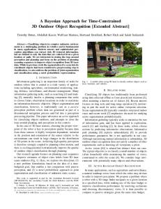
Figure 1: Example of real data from the COIL-20 database. The two basis view images I 0 (a) and I 00 (b) with landmark points selected at prominent features. IT (c) is the target image. The synthesised image IS (d) is at the correct pose identified by our algorithm.

Linear combination of views

LCV is a technique which belongs in the general theory of the tri- and multi-focal tensors, or Algebraic Function of Views (AFoV) (Shashua, 1995) and provides a way of dealing with variations in an object’s appearance due to viewpoint changes. This theory is based on the observation that the geometry of the set of possible images of an object undergoing 3d rigid transformations and scaling may, under most imaging conditions, to a good approximation, be embedded in a linear space spanned by the landmark points of a small number of images taken from different viewpoints. Ullman and Basri (Ullman and Basri, 1991) were the first to apply this theory to line drawings and edge maps. Thus, given two images I 0 and I 00 of an object from different (basis) views with corresponding image coordinates (x0 , y0 ) and (x00 , y00 ), we can represent any corresponding point (x, y) in a novel target image IT according to, for example: x = a0 + a1x0 + a2y0 + a3x00 + a4y00 . y = b0 + b1x0 + b2y0 + b3x00 + b4y00

(1)

The target view is reconstructed from the above two equations given a set of valid coefficient (ai , b j ). Provided we have at least 5 corresponding landmark points in all three images (IT , I 0 , I 00 ) we can estimate the coefficients (ai , b j ) by using a standard least squares approach. Several others have taken this concept further from its initial application to line images and edge maps to the representation of real images IT (Bebis et al., 2002; Koufakis and Buxton, 1998; Hansard and Buxton, 2000; Peters and von der Malsburg, 2001).

Such results suggest that it is possible to use LCV for recognition by matching images IT of target views of an object to a combination of stored, basis views of the object. The main difficulty in applying this idea within a pixel-based approach is the selection of the LCV coefficients (ai , b j ).

2.1 Image synthesis To synthesise a single, target image using LCV and two views we first need to determine its geometry from the landmark points. For pixel-based object recognition in which we wish to avoid feature detection a direct solution is not possible, but we instead use a powerful optimisation algorithm to search and recover the LCV coefficients for the synthesis. Given a set of hypothesised landmark points (see Fig. 1(a),(b)) we can, to a good approximation, synthesise an image IS to match to the target IT : IT (x, y) = w0 I 0 (x0 , y0 ) + w00 I 00 (x00 , y00 ) + ε(x, y) = IS (x, y) + ε(x, y).

(2)

The weights w0 and w00 may be calculated from the LCV coefficients and the image IS synthesised as described in (Koufakis and Buxton, 1998). Thus, 002 02 w0 = d 02d+d 002 , w00 = d 02d+d 002 with d 002 = a23 + a24 + b23 + b24 + a20 + b20 and d 02 = a21 + a22 + b21 + b22 + a20 + b20 . The synthesis essentially warps and blends images I 0 and I 00 to produce IS . It is important to note therefore that (2) applies to all points (pixels) (x, y), (x0 , y0 ) and (x00 , y00 ) in images IS , I 0 and I 00 with the dense correspondence defined by means of the LCV equations

(1) and a series of piecewise linear mappings (Goshtasby, 1986; Koufakis and Buxton, 1998). If (x0 , y0 ) and (x00 , y00 ) do not correspond precisely to pixel values, bilinear interpolation is used. The same idea may be extended to colour images by treating each spectral band as a luminance component (e.g. IR , IG , IB ).

2.2 Coefficient variation Since the pose information is implicitly encoded in the 10 coefficients (ai , b j ), it is useful to investigate their variation as the object is viewed from different directions. We are particularly interested in viewing directions on the portion of the view-sphere between the two basis views. We thus devised a simple experiment using a synthetic 3d model on which we selected a number of landmarks on prominent features and along edges. The model was placed over a black background and then allowed to rotate between ±20o from the frontal position and 2d snapshots of the scene were taken, under orthographic projection, at 1o intervals. The two images at ±20o were chosen as the basis views. We then solved (1) at each view and obtained a set of coefficients as a function of the angle ϑ as illustrated in Fig. 3(b). As we can see, coefficient a0 follows a quadratic curve, coefficients a1 and a3 are linear and the remaining coefficients are constant. Note also that a1 and a3 have a range of [0, 1] with a1 , a3 ≈ 0.5 for ϑ = 0o (frontal view). Additionally, at the same angle, a0 is at a minimum. Finally, we observe that, a2 , a4 , b0 , b1 , b3 ≈ 0 and b2 , b4 ≈ 0.5 . This information could be used to bound the parameter space in the optimisation or to approximate regions within which we initialise our algorithm. Alternatively, we can predict the solution set at each ϑ. This information, combined with knowledge of the range of poses we are likely to encounter in a specific experiment, may thus be used to construct the Bayesian priors, as we shall see in section 3 We note here that the form of the coefficients is largely independent of the actual object used and therefore the results generalise to any generic object under similar imaging conditions. One could also carry out similar experiments with other 3d rigid transformations and recover how the LCV coefficients vary in such cases.

3

Bayesian model

In this section we propose an extension of the basic LCV equations (1) and (2) by incorporating prior information on the coefficients (ai , b j ) and building a

Bayesian model. We start with (2) in which ε(x, y) is assumed to be a vector of i.i.d. random noise. Given the data (target image IT ) and a model represented by the basis views I 0 and I 00 , the posterior probability of the LCV coefficients is: P(ai , b j |IT , I 0 , I 00 ) ∝ P(IT |ai , b j , I 0 , I 00 )P(ai , b j ).

(3)

P(IT |ai , b j , I 0 , I 00 ) is the probability of observing the target image IT given the coefficients (ai , b j ) and the basis views I 0 and I 00 . P(ai , b j ) is the prior probability of the LCV coefficients. If we then use the general assumption that the deviations ε of the synthesised image IS from the target image IT are drawn from a Gaussian distribution the log-likelihood of observing the target image may, up to constant terms that we shall ignore, be written as: − log[P(IT |ai , b j , I 0 , I 00 )] = 1 ∑ [I (x, y) − IS (x, y)]2 , 2σ2 x,y T

(4)

ε

which is quadratic in the residuals, and the summation is over all image pixels. The other term on the right in (3) comes from the prior p.d.f.. The prior represents general information about the LCV parameters based on the analysis we have carried out previously. We have used a Gaussian prior for the coefficients ai and b j centered at the values identified in section 2.2. Under the assumption of statistical independence of the coefficients with each having its own mean and variance and, if we again ignore uninteresting constants we get: 4

(ai − µa)2 (b j − µb )2 + ], σ2i σ2j i, j=0 (5) where µa , µb are the means and σi ,σ j the standard deviations of the prior probabilities for coefficients ai and b j respectively. From (3),(4) and and (5) we see that, if we continue to ignore uninteresting constants, the log posterior probability becomes: − log(P(ai , b j )) ∝

∑[

− log[P(ai , b j |IT , I 0 , I 00 )] ∝ ∑x,y [IT (x,y)−IS (x,y)]2 σ2ε

2

a) + ∑4i, j=0 [ (ai −µ + σ2 i

(b j −µb )2 ]. σ2j

(6) We usually require a single synthesised image to be presented as the most probable result. A typical choice for that single image is the one which maximises the posterior probability (MAP), or minimises the negative log-posterior (6) with respect to the parameters ai and b j . The latter can be minimised using standard optimisation techniques. As we can see from (6), the prior is used to bias the MAP solution toward the means µa and µb , away

from the maximum likelihood (ML) solution which is where ∑x,y [IT (x, y) − IS (x, y)]2 is at a minimum (i.e. there is little difference between IT and IS ). How much the prior affects the solution in relation to the likelihood depends on the ratio: k=

σ2ε . ∑i, j (σ2i + σ2j )

(7)

As the influence of the prior vanishes (i.e. σi , σ j become very big and the Gaussian prior resembles a uniform distribution) the MAP solution approaches the ML solution. Careful selection of the ratio k is therefore very important. The effect of using such Gaussian priors to bias the posterior can be seen in Fig. 3(a). Here we show the negative log probability of the likelihood, prior and posterior for the coefficient a2 . This plot was generated by isolating and varying this coefficient while having conditioned the remaining coefficients to the optimal prior values identified previously. The image IS was synthesised using (2) and compared to the target image IT with the log probabilities recorded at each value of a2 . We used images from the COIL-20 database (Nene et al., 1996). What we should note in particular from this example is the effect of the prior on the likelihood, especially near the tails of the p.d.f. where we have large error residuals. The prior widens the basin of attraction of the likelihood resulting in a convex posterior that is much easier to minimise even if we initialise our optimisation algorithm far away from the optimal solution. On the other hand, near the global optimum we wish the prior to have as little impact as possible in order for the detailed information as to the value of a2 to come from the likelihood. This allows for small deviations from the values for the coefficients encoded in the prior means, since every synthesis and recognition problem differs slightly, due to object type, location, orientation and perspective camera effects.

4

The recognition system

In principle using the LCV for object recognition is straightforward. All we have to do is select the object and find the coefficients in an equation such as (1) which will minimise the error ε from (2) and check that it is small enough so that our synthesised and target images IS and IT are sufficiently similar to enable us to say that they match.

4.1 Template matching The first component of our system is the two stored basis views I 0 and I 00 which define the library of known modelled objects. These are rectangular bitmap images that contain grey-scale (or colour) pixel information of the object without any additional background data. It is important not to choose a very wide angle between the basis views to avoid I 0 and I 00 belonging to different aspects of the object with landmark points being occluded. Having selected the two basis views, we pick a number of corresponding landmark points, in particular lying on edges and other prominent features. We then use constrained Delaunay triangulation (Shewchuk, 2002) and the correspondence to produce similar triangulations on both the images. The above processes may be carried out during an off-line, model-building stage and are not examined here. The set of LCV coefficients is then determined by minimising the negative log posterior (6) and the object of interest in the target image IT recognised by selecting the best of the models, as represented by the basis views, that explain IT sufficiently well. Essentially, we are proposing a flexible template matching system, in which the template is allowed to deform in the LCV space, restricted by the Bayesian priors to regions where there is a high probability of meaningful solutions, until it matches the target image.

4.2 Optimisation To recover the LCV coefficients, we need to search a high-dimensional parameter space using an efficient optimisation algorithm. For this purpose, we have chosen to examine two different methods, a global, stochastic algorithm, and a local, direct-search approach. The stochastic method used is called Differential Evolution (DE) and was introduced by (Storn and Price, 1997). Briefly, DE works by adding the weighted difference between two randomly chosen population vectors to a third vector, and the fitness of the solution represented by the resultant is compared with that of another individual from the current population. For the local method, we have selected the simplex algorithm by (Nelder and Mead, 1965) since it is very easy to implement and does not require calculation (or approximation) of first or second order derivatives. A simplex is a polytope of N+1 vertices in N dimensions with each vertex corresponding to a single matching function evaluation. In its basic form the simplex is allowed to take a series of steps, the most common of which is the reflection of the vertex

Figure 2: Image samples from the COIL-20 database

having the poorest value of the objective function. It may also change shape (expansion and contraction) to take larger steps when inside a valley or flat areas, or to squeeze through narrow cols. It can also change direction (rotate) when no more improvement can be made in a current path. Since the simplex is a local, direct search method it can become stuck in local optima and therefore some modifications of its basic behaviour are necessary. We thus introduced the reducing-step restarting simplex (Zografos and Buxton, 2007) which can make variable length “jumps” in order to avoid local optima and burrow deeper into the basin of attraction.

5

Experiments

We have performed a number of experiments on real images using the publicly available COIL-20 database. This database contains examples of 20 objects imaged under varying pose (horizontal rotation around the view-sphere at 5o intervals) against a constant background with the camera position and lighting conditions kept constant (see Fig. 2). We constructed LCV models from 5 objects, using as basis views the images at ±20o from a frontal view, while ensuring that the manually chosen landmarks were visible in both I 0 and I 00 (Fig. 1). Comparisons were carried out against target images from the same set of modelled objects taken in the frontal pose at 0o . In total, we carried out 500 experiments (250 with each optimisation method × 10 tests for each modeltarget image combination) and constructed two 5 × 5 arrays of model×image results. Each array contains information about the matching scores represented by the cross-correlation coefficient (Zografos and Buxton, 2007). The highest scores were along the main diagonal, where each model of an object is correctly matched to a target image of the same object. The

recognition response should be less (or have a higher negative log probability) when comparing a specific model with images of other objects. For the simplex method, we set the maximum number of function evaluations (NFEs) to 1000 and a fixed initialisation of: ao ,a1 ,a3 ,b0 ,b1 =1, a2 ,a4 ,b3 =0.5, b2 =0.9, b4 =1.4, deliberately chosen far away from the expected solution, in order not to influence the optimisation algorithm with a good initialisation. In the case of DE, we chose a much higher NFEs=20000 (100 populations × 200 generations) and specified the boundaries of the LCV space as: -5≤ a0 , b0 ≤5, 1≤ a1 ,a2 ,a3 ,a4 ≤1, -1≤ b1 ,b2 ,b3 ,b4 ≤1. This includes the majority of the coefficient ranges identified in section 2.2. The results of the above experiments, averaged over 10 test runs, are summarised in the heatmap plot Fig. 3(c). As expected, we can see a well defined diagonal of high cross-correlation where the correct model is matched to the target image. This observation, combined with the absence of any significant outlying good matches when model6=image, leads us to the conclusion that, on average, both methods perform equally well in terms of recognition results. The only difference is how close these methods can get to the global optimum, and in how many NFEs. To explore this further, we have included the plot in Fig. 4 which compares the average crosscorrelation responses for both methods. We observe that both methods have a consistently good performance, with the DE converging to solutions of higher cross-correlation in the majority of cases. The simplex failed to converge to the correct solution in a few cases, particularly in some of the tests for models 1 and 9. This of course may be explained in part by the smaller NFEs that were allowed for this algorithm, although preliminary experiments had indicated the NFE value chosen should generally have sufficed. We also include boxplot diagrams, Fig. 3(d),(e), which illustrate the diversity of the 10 coefficients in the recovered solutions. For this, results were taken from the test runs along the main diagonal, using both of the optimisation algorithms. We can see that there is little diversity in the coefficients with few or no outliers, indicating a stability in the values already identified by the 3d experiment (section 2.2) across different objects. The only significant variation is, as expected, in the translation coefficients a0 and b0 . Finally, we have included in Fig. 3(g),(h) for test runs on the main diagonal when the correct model is matched to a target image, values of the negative log probability as the number of function evaluations increases. From these, we observe the different optimisation behaviours of the two algorithms, DE and

simplex, and how much earlier the latter can reach the global minimum. DE is much slower, but it has the advantage that it can avoid locally optimum solutions, which the simplex sometimes clearly cannot.

5.1 Markov-Chain Monte-Carlo In previous sections we have introduced the posterior distribution and have provided some graphs of the variation of the individual coefficients. Nevertheless, graphical analysis of the 10-dimensional posterior distribution is difficult, so to obtain a more specific and complete idea of its characteristics we have used a Markov-Chain Monte Carlo (MCMC) (Gelman et al., 1995) approach in order to generate a sample of the distribution and further analyse it. Briefly, MCMC is method for sampling from an unknown distribution, requiring only that its density can be calculated at each point. Initially MCMC draws values from a known, starting distribution and then gradually adjusts these draws to converge to an approximation of the posterior distribution. These samples are drawn sequentially with the draws forming a Markov Chain. In this particular implementation, we have used the Metropolis-Hastings rule (Metropolis et al., 1953; Hastings, 1970) and a product of ten 1-dimensional normal distributions, such as those used in section 3 for the priors, as a starting distribution. In addition, the first half of the samples were discarded in order to reduce any residual correlation in the draws. We chose a single experiment (matching to a frontal view of object 1 at 00 ) and generated a set of 10000 samples of the posterior (6) from areas of high probability using a single Markov Chain. The MCMC converged to a point very close to the global optimum, with a cross-correlation of 0.98508 (the best solution recovered by the simplex was 0.987301 and that for the DE was 0.973954). The way the MCMC gradually improved the posterior probability can be seen in Fig. 3(i) and compared with the simplex and DE methods illustrated in Fig. 3(g) and (h). The first step of the analysis is to determine the major modes of the p.d.f. and find where other locally optimal solutions may be situated. For that purpose, we used repeated runs of a k-means clustering algorithm (Bishop, 1995), the best of which recovered 3 main clusters in close proximity and all near the global optimum. This leads to the conclusion that the distribution has a single mode (i.e. peak) perhaps with some subsidiary, nearby peaks caused by noise effects. The main point is that there is no significant local optimum elsewhere nearby in the distribution. We have also included boxplots of the samples of

the LCV coefficients taken in the MCMC in Fig. 3(f). The samples are tightly bundled with a few outliers, another indication that the algorithm has converged to the optimum. This reinforces the notion that the posterior distribution we have constructed is unimodal. For a quantitative, numerical analysis we have calculated the statistical characteristics of the coefficients a0 − a4 , b0 − b4 produced by the MCMC sampling as shown in Table 1. The characteristics of the coefficients a0 − a4, b0 − b4 described in the first two columns are arranged in two rows in the last five columns of the table. Our first observation is that the means, modes and medians of each of the coefficients almost coincide, consistent with the posterior being an approximately symmetric, unimodal distribution. If we look at the range values, we see once more that the values are tightly concentrated signifying a basin of attraction that bottoms-out into a few close-by points. This is further affirmed by the low standard deviations of the sampled values of all 10 coefficients. If we now examine the kurtosis and skewness we can see positive skewness in the samples of certain coefficients and negative in others. The distributions of the samples of all coefficients, except b1 , are quite strongly skewed, reflecting strong influence of the likelihood near the optimum posterior, a property that is highly desirable. This is due to the shape of the likelihood function since the priors are symmetric. The values for the kurtosis are small for some coefficients whose posteriors are therefore almost Gaussian near the optimum, whilst other coefficients strongly affected by the priors are leptokurtic, in particular a4 , b2 and b4 .

6

Conclusion

We have shown how the linear combination of views (LCV) method may be used in view-based object recognition. Our approach involves synthesising intensity images using LCV and comparing them to the target, scene image. In addition, we incorporate prior probabilistic information on the LCV parameters by means of a Bayesian model. For the priors, we chose Gaussian distributions centered at the expected values of those parameters given a specific transformation (in this case rotation of the object about a vertical axis in 3d). Matching and recognition experiments were then carried out on data from the COIL-20 public database using two different optimisation algorithms in order to recover the optimal LCV parameters. These experiments have shown that our method works well for

k=64

x 10

−log probability

8

1

a

3

1

0.9

a

Likelihood Prior Posterior

2

2

a

3

6

1

a

0

b

0

b

1

−1

b

4

3

0.8

5

0.7

4

Model

4

10

2

−2

0.6

b

3

2

0 −2

−1

0

1

2

3

−3

b

−4

a

0.5

0

−5 −20

4

7

4

−10

a2

0

10

9 1

20

Angle

(a)

3

5

DE. Averaged over test runs.

9

Image

(b)

(c)

Simplex. Averaged over test runs.

2

7

MCMC Model = Image = 1

1.5 1 0.8

−1

Value

1

0

Value

Value

1

0.5

0.6 0.4

−2 0.2 −3

0

0

a0 a1 a2 a3 a4 b0 b1 b2 b3 b4

a0 a1 a2 a3 a4 b0 b1 b2 b3 b4

a0 a1 a2 a3 a4 b0 b1 b2 b3 b4

Coefficient

Coefficient

Coefficient

(d) 4

5

x 10

(e)

Simplex. Model=Image

4

x 10

(f)

DE. Model=Image

3 2 1 0 0

200

400

600

800

4

−log probability

−log probability

−log probability

4

MCMC. Model=Image=1

4

x 10

4 3 2 1 0 0

0.5

1

1.5

Function evaluation

Function evaluation

(g)

(h)

3 2 1 0 0

2

2000

4000

6000

8000

10000

Function evaluation

4

x 10

(i)

Figure 3: (a) The negative log posterior resulting from the combination of the prior and likelihood. (b) Variation plot of the 10 LCV coefficients. (c) Model x Image heatmap array with high cross-correlation on the main diagonal. (d)-(f) Coefficient diversity plots for the DE, Simplex and MCMC methods respectively. (g)-(i) Iterative optimisation results for the three methods. Note the different scales on the ordinate and the vertical line in (h) indicating the NFEs for the simplex method. Table 1: Statistical characterisation of the MCMC algorithm.

Dispersion measures: range std. dev.

a0 : b0 : a0 : b0 :

0.069 0.045 0.013 0.015

a1 : b1 : a1 : b1 :

0.072 0.058 0.024 0.006

a2 : b2 : a2 : b2 :

0.038 0.037 0.015 0.008

a3 : b3 : a3 : b3 :

0.034 0.009 0.012 0.002

a4 : b4 : a4 : b4 :

0.036 0.043 0.010 0.004

a0 : b0 : a0 : b0 : a0 : b0 :

1.050 0.981 1.042 0.972 1.042 0.972

a1 : b1 : a1 : b1 : a1 : b1 :

0.551 -0.004 0.564 -0.005 0.564 -0.005

a2 : b2 : a2 : b2 : a2 : b2 :

-0.031 0.481 -0.040 0.480 -0.040 0.480

a3 : b3 : a3 : b3 : a3 : b3 :

0.474 -0.000 0.467 0.001 0.467 0.001

a4 : b4 : a4 : b4 : a4 : b4 :

0.016 0.510 0.022 0.510 0.022 0.510

a0 : b0 : a0 : b0 :

1.171 1.3685 -0.568 0.193

a1 : b1 : a1 : b1 :

-1.458 0.305 0.309 1.523

a2 : b2 : a2 : b2 :

1.214 2.520 -0.466 6.325

a3 : b3 : a3 : b3 :

1.275 -1.689 -0.256 0.874

a4 : b4 : a4 : b4 :

-2.053 -2.071 3.301 5.668

Location measures: mean median mode Distributional measures: skewness kurtosis (-3)

Responses averaged over test runs

Gelman, A., Carlin, J. B., Stern, H. S., and Rubin, D. B. (1995). Bayesian Data Analysis. Chapman and Hall, London, 2nd edition.

0.96

Cross correlation

0.94

Goshtasby, A. (1986). Piecewise linear mapping functions for image registration. 19(6):459–466.

0.92 0.9

Hansard, M. E. and Buxton, B. F. (2000). Parametric viewsynthesis. In Proc. 6th ECCV, 1:191–202.

0.88

Hastings, W. (1970). Monte carlo sampling methods using markov chains and their applications. Biometrika, 57(1):97–109.

0.86 DE

0.84

Simplex 0.82 1

3

5

7

9

Model

Figure 4: Comparison of the average response between the DE and simplex algorithms.

pose variations where the target view lies between the basis views. The experiments further show the beneficial effects of the prior distributions in “regularising” the optimisation. In particular, priors could be chosen that produced a good basin of attraction surrounding the desired optimum without unduly biasing the solution. Finally, we used MCMC to draw a sample from the posterior distribution and carried out additional tests to characterise the shape of the distribution. The use of the MCMC approach as an optimisation solution was also briefly explored with, because of the form of the posterior, satisfactory results. Nevertheless, additional work is required. The kurtosis of the posterior distribution calculated from the samples taken in the MCMC experiment suggests that there may be effects arising from the fact that the LCV coefficients are not all independent. We would thus like to reformulate the LCV equations (1) by using the affine tri-focal tensor and introducing the appropriate constraints in the LCV mapping process. In addition, in this paper we have only addressed extrinsic viewpoint variations, but it should also be possible to include intrinsic, shape variations using the approach described by (Dias and Buxton, 2005).

Koufakis, I. and Buxton, B. F. (1998). Very low bit-rate face video compression using linear combination of 2dfaceviews and principal components analysis. Image and Vision Computing, 17:1031–1051. Lamdan, Y., Schwartz, J., and Wolfson, H. (1988). On recognition of 3d objects from 2d images. Proceedings of the IEEE International Conference on Robotics and Automation, pages 1407–1413. Lee, M. W. and Ranganath, S. (2003). Pose-invariant face recognition using a 3d deformable model. Pattern Recognition, 36:1835–1846. Li, W., Bebis, G., and Bourbakis, N. (2004). Improving 3d object recognition based on algebraic functions of views. Metropolis, A., Rosenbluth, W., Rosenbluth, M., Teller, H., and Teller, E. (1953). Equation of state calculations by fast computing machines. J. Chem. Phys., 21(6):1087–1092. Nelder, J. A. and Mead, R. (1965). A simplex method for function minimization. Computer Journal, 7:308– 313. Nene, S. A., Nayar, S. K., and Murase, H. (1996). Columbia Object Image Library (COIL-20). Technical Report CUCS-006-96, Department of computer science, Columbia University, New York, N.Y. 10027. Peters, G. and von der Malsburg, C. (2001). View reconstruction by linear combination of sample views. In Proc. British Machine Vision Conference BMVC 2001, 1:223–232. Shashua, A. (1995). Algebraic functions for recognition. IEEE Transactions on Pattern Analysis and Machine Intelligence, 17(8):779–789.

REFERENCES

Shewchuk, J. R. (2002). Delaunay refinement algorithms for triangular mesh generation. Computational Geometry: Theory and Applications, 22:21–74.

Bebis, G., Louis, S., Varol, T., and Yfantis, A. (2002). Genetic object recognition using combinations of views. IEEE Transactions on Evolutionary Computation, 6(2):132–146.

Storn, R. and Price, K. V. (1997). Differential evolution - a simple and efficient heuristic for global optimization overcontinuous spaces. Journal of Global Optimization, 11(4):341–359.

Beymer, D. J. (1994). Face recognition under varying pose. In Proc. IEEE Conf. CVPR, pages 756–761.

Ullman, S. and Basri, R. (1991). Recognition by linear combinations of models. IEEE Transactions on Pattern Analysis and Machine Intelligence, 13(10):992–1006.

Bishop, C. M. (1995). Neural Networks for Pattern Recognition. Oxford University Press. Dias, M. B. and Buxton, B. F. (2005). Implicit, view invariant, linear flexible shape modelling. Pattern Recognition Letters, 26(4):433–447.

Zografos, V. and Buxton, B. F. (2007). Pose-invariant 3d object recognition using linear combination of 2d views and evolutionary optimisation. ICCTA, pages 645–649.