374
IEEE TRANSACTIONS ON BIOMEDICAL ENGINEERING, VOL. 44, NO. 5, MAY 1997
A Bayesian Approach to Introducing Anatomo-Functional Priors in the EEG/MEG Inverse Problem Sylvain Baillet* and Line Garnero Abstract— In this paper, we present a new approach to the recovering of dipole magnitudes in a distributed source model for magnetoencephalographic (MEG) and electroencephalographic (EEG) imaging. This method consists in introducing spatial and temporal a priori information as a cure to this ill-posed inverse problem. A nonlinear spatial regularization scheme allows the preservation of dipole moment discontinuities between some a priori noncorrelated sources, for instance, when considering dipoles located on both sides of a sulcus. Moreover, we introduce temporal smoothness constraints on dipole magnitude evolution at time scales smaller than those of cognitive processes. These priors are easily integrated into a Bayesian formalism, yielding a maximum a posteriori (MAP) estimator of brain electrical activity. Results from EEG simulations of our method are presented and compared with those of classical quadratic regularization and a now popular generalized minimum-norm technique called low-resolution electromagnetic tomography (LORETA). Index Terms— Bayesian imaging, EEG, edge-preserving regularization, MEG, multimodality imaging, source estimation.
I. INTRODUCTION
A
S a tool for human brain mapping of cognitive functions, functional brain imaging long-term objectives are twofold: localizing groups of neurons involved in some simple cognitive tasks such as those dealing with a perceptual process, and then identifying dynamic links between these groups in order to hopefully better understand “how does the brain work?” [1]. Once the problem is put in such a way, it is obvious that functional imaging modalities should ideally offer excellent space and time resolutions. Defining space and time resolution is not an easy task and may still be considered as an open issue. Nevertheless, spatial and temporal accuracy should be at least better than 5 mm and 5 ms, respectively. Current functional brain imaging techniques such as position emission tomography (PET), single photon computed tomography (SPECT), and functional magnetic resonance imaging (f-MRI) possess excellent spatial resolutions but fail to offer, Manuscript received March 15, 1996; revised December 30, 1996. Asterisk indicates corresponding author. *S. Baillet is with the Unit´e de Psychophysiologie Cognitive, Hˆopital de la Salpˆetri`ere, CNRS URA 654, LENA—Universit´e Paris VI, Paris, France. He is also with the Institut d’Optique Th´eorique et Appliqu´ee, CNRS URA 14—Universit´e Paris XI, Facult´e d’Orsay, Orsay, France (e-mail:
[email protected]). L. Garnero is with the Unit´e de Psychophysiologie Cognitive, Hˆopital de la Salpˆetri`ere, CNRS URA 654, LENA—Universit´e Paris VI, Paris, France. She is also with the Institut d’Optique Th´eorique et Appliqu´ee, CNRS URA 14—Universit´e Paris XI, Facult´e d’Orsay, Orsay, France. Publisher Item Identifier S 0018-9294(97)02956-X.
at the same time, temporal resolution better than, say, 1 min in PET/SPECT and 1 s in f-MRI [2], [3]. This time limitation is mainly due to metabolic considerations, like the evolution of radioactive isotope concentration in blood with PET and SPECT. f-MRI time resolution is still very promising, but technical problems remain. Electromagnetic imaging of the brain is the only functional imaging modality that is liable to offer excellent time resolution. In principle, one could be able to obtain functional images of the brain electrical activity up to every millisecond (which roughly corresponds to the data sampling rate). Unfortunately, spatial resolution is limited and moreover, very different source arrangements can lead to the same electroencephalographic (EEG) and magnetoencephalographic (MEG) measurements. Owing to this nonuniqueness and also to numerical instability, the inverse problem consisting in finding out a source map from data is said to be ill posed. Many researchers have proposed methods to regularize this issue. Very often, these latter consist in finding one or two best-fitting current dipoles according to data or, while using a distributed source model, give minimum-norm solutions characterized by spatial over-smoothing. These methods do not explicitly introduce anatomical or physiological constraints in the source reconstruction process, and so may yield unrealistic solutions. In this paper, we propose an inversion method that introduces some a priori information and works out at some spatio-temporal regularization. For instance, when consistent with physiology, we show how it may be possible to introduce discontinuities between magnitudes of sources located on both sides of a sulcus. We also introduce temporal smoothness constraints on source intensities with respect to the data sampling rate. We particularly insist on the fact that this spatiotemporal information yields better and less time consuming results than spatial regularization only. This paper is divided as follows: in Section II, we review the formalism of the inverse problem with a distributed source model and briefly describe the different approaches currently in use. In Section III, we expose the a priori information we wish to introduce in the reconstruction process. These spatio-temporal priors result from multimodal registration of magnetic resonance imaging (MRI) and PETor f-MRI images. In Section IV, we show how it is possible to introduce such an information in a Bayesian formalism with a maximum a posteriori (MAP) estimator of dipole activities. Then we describe a nonoptimal and deterministic algorithm used to achieve a minimum of the energy function associated to the
0018–9294/97$10.00 1997 IEEE
BAILLET AND GARNERO: INTRODUCING ANATOMO-FUNCTIONAL PRIORS IN THE EEG/MEG INVERSE PROBLEM
Gibbs formulation of the conditional probability distribution of dipole magnitudes given the data. Section V describes concisely the quadratic regularization (QR) and the generalized minimum-norm [low-resolution electromagnetic tomography (LORETA)] methods that will be used in Section VI, where results from a simulated auditory experiment are shown and compared with both those from the QR and LORETA methods. II. EEG/MEG SOURCE IMAGING AS AN INVERSE PROBLEM The idea of using EEG and MEG as genuine brain imaging techniques is quite simple [4], [5]. There are two complementary ways to measure the electromagnetic signature of the neural electric activity outside the skull: cutaneous electrodes measuring electric potentials—EEG; supraconductive coils measuring some components of the magnetic field on the surface of the head—MEG. Thus, one can investigate whether it is possible to reconstruct neural ionic currents as sources of these data. Fundamentally, the main asset of EEG/MEG imaging is that one could obtain a mapping of neuronal electric activity with the same time resolution as the data sampling rate (typically 1–4 ms). In a distributed source model using current dipoles with given positions and orientations, it is possible to gather all the sources in a row vector so as to obtain the following linear system: (1) is a row vector containing (EEG or MEG) where measurements at time , and is a matrix containing global information about the head model, the source set pattern, and measurement positions on the surface of the skull. is a row vector containing the th time sample of dipole magnitudes. Finally, data are corrupted by an additive measurement noise . This is a standard writing for many linear forward problems in image reconstruction. Thus, the matrix and the source positions make up a framework for the following inverse problem: find the sources that best explain the EEG and/or MEG measurements. It is well known that this is an ill-posed problem. • The Solution is Not Unique: Radically different source configurations may offer the same excellent fit to data. Moreover, dipoles radially oriented with regards to the surface of the skull are “silent” in MEG measurements. • The Solution is Not Stable: As matrix is nearly singular, or in other words the linear system associated to (1)—i.e., —is ill conditioned [38], there is little control over the propagation of measurement errors from the data to the solution. Regularization techniques are applied so as to counter the bad conditioning of the linear operator by introducing complementary information on parameters to be estimated [7]–[9]. Owing to nonuniqueness, the problem should be confined to one for which the solution space dimension is reduced by the introduction of restricting criteria. The first approach consists in searching for a single or few dipoles whose forward solution to (1) is a best fit (generally in a least squares sense) to measurements [10], [11]. Another technique can be found in
375
[14], where Mosher et al. propose a method derived from the widely used antenna processing multiple signal classification algorithm (MUSIC, [15]), which consists in estimating the active source locations by computing the projection of a fixed number of current dipoles onto the noise subspace of the measurement space. Greenblatt in [16] proposes an extension of this method to the case where there are more expected sources than measurement data, so there is no possible subspace decomposition of measurement space. His method consists in building a metric based on the covariance matrix estimated from data time slices. Then, the source space is projected through this metric onto the measurement space. A weighted forward matrix is computed via a singular value decomposition (SVD) of the matrix whose columns are the projections, through this metric, of the original source space basis onto the measurement space. This yields estimated source locations that mostly contribute to the signal component in data. The final result is a weighted pseudo-inverse of the forward matrix scanning through data time series to estimate sources. In [12], a minimum-norm solution to (1) using a distributed source model (i.e., ) is proposed. Recently PascualMarqui et al. have presented a generalized minimum-norm solution to the inverse problem that appears to overcome some of the limitations of other minimum-norm methods that tend to yield solutions with most of the active dipoles at the surface of the source space as a priority (because of the decrease of lead field intensities with depth, see Section V) [13]. As a primary conclusion, it appears that most of the time, single dipole models fail to give acceptable results when space and time overlapping in the source pattern is very likely. That is especially the case with the late components of evoked potentials where unique dipole models may yield inconsistent solutions in regard to physiology [17]. On the other hand, distributed sources minimum-norm solutions have over-smoothed magnitude patterns and do not respect specific brain anatomical constraints like sulcus borders. In [18], one can find a first attempt to constrain solutions on anatomical surfaces, deduced from a preliminary MRI study of the subject, which greatly improves the quality of the solution. Such an approach has been extensively used in a recent CURRY source reconstruction software in which one has the possibility to constrain dipoles perpendicularly to the cortex surface [19]. What we propose here is to introduce some additional a priori information into the regularization process so as to obtain the most probable and satisfying solution in regard to some physiological and anatomical criteria in connection with a given cognitive experiment. III. WHAT KIND OF RELEVANT SPATIO-TEMPORAL A PRIORI INFORMATION COULD BE INTRODUCED? In this section, we make an overview of the a priori assumptions we make while searching for a physiologically consistent solution to the EEG/MEG inverse problem. A. Anatomical Constraints What we propose here is to reduce the dimension of the source space by introducing anatomical constraints on dipole
376
IEEE TRANSACTIONS ON BIOMEDICAL ENGINEERING, VOL. 44, NO. 5, MAY 1997
won’t describe here—in order to obtain effective data fusion between those different imaging techniques. In addition to those anatomical constraints, we make some further spatiotemporal assumptions on dipole magnitudes distribution and evolution according to physiology. B. Physiological Constraints
Fig. 1. Cortex patches representing a priori brain active areas isolated owing to anatomical MRI and PET imaging in an auditory experiment. These patches are located in temporal auditive and motor cortex areas. (NI) is the Nasion–Inion line. Black dots on every patch are for dipole locations.
locations and orientations. Such an approach has already been adopted by researchers and is becoming widely used [18]–[20]. The main motivation is to prevent solutions from being found in unrealistic locations (i.e., in the white matter for instance). In our method, we propose an extension of Dale and Sereno’s approach which consists in distributing dipoles on the cortex surface owing to high-resolution MRI anatomical images. Moreover, we adopt the same restricting hypothesis as in [18] by demanding that dipoles have fixed orientations but changing magnitudes during a given experiment. More precisely, we use the fact that the only neuronal electric activity that can be measured outside the skull by EEG and MEG comes mainly from groups of neurons organized in macrocolumns perpendicularly to the cortex surface [21]. Once these assumptions are made, we build a distributed source model as a patchwork where dipoles are distributed on little surfaces that locally approximate some parts of the cortex surface. These patches are located using previous PET or f-MRI experiments with the same subject, resulting in “average” images of active brain areas during a given task. This means we make the strong assumption that metabolically active areas are closely related to active neuron groups [22]. As an example, Fig. 1 shows active areas isolated from PET data in an auditory experiment [23]. A priori active areas may also be deduced from cognitive considerations, allowing the introduction of fugitive sources in areas that will not appear on any metabolic imaging modality. Here, the source space is designed with “patches” that are tangent to the cortex surface. It is then possible to distribute dipoles on these planes so as to create the source space. The number of dipoles per plane may vary, and could be proportional to the patch surface for instance. Such a modelization needs an accurate multimodal registration procedure—which we
We introduce two supplementary constraints as follows: first, one can safely consider that relevant frequencies of neural electrical activity are inferior to 100 Hz, and since measurements are over sampled, it is assumed that dipole magnitude evolution is smooth in time. In Section IV, we will see how this prior can be introduced as some kind of a temporal lowpass filter on . Second, although we assume that dipoles on the same surface patch have strongly related activities, it could also be possible that dipoles located on two different surface patches have completely separated activities. For instance, one can suppose that activities of dipoles located on two different walls of a sulcus, in some cases, could be very functionally noninterdependent depending on the nature of physiological constraints. As a conclusion, these priors lead to the idea that the source space is made of locally homogeneous and smoothly time evolving areas (cortex patches) that can be considered partially or totally independent from one to another depending on physiological aspects. After having created some spatio-temporal neighborhood for each dipole—and when considering dipole magnitudes as pixel intensities of a reconstructed image—assuming noncorrelated activities between some dipoles means that discontinuities may exist in the source image despite the fact that most of the inversion techniques produce spatially over-smoothed solutions. This over smoothing is due to the usual practice to operate some kind of spatial lowpass filtering onto the reconstructed image, in order to make the balance right between algorithmic stability (noise averaging by some spatio-temporal lowpass filter) and information preservation. As a lot of informative contents usually lie in higher frequency ranges—like plosive consonants in many languages and sharp edges in pictures—one can imagine that a compromise is to be found in some kind of adaptive filtering. In order to break free from this and to proceed with a selective image filtering, we show in Section IV that all the previous spatio-temporal a priori information can easily be introduced in a Bayesian framework while using a MAP estimator of dipole magnitudes. More particularly, we will see that it is possible to regularize this inverse problem while, at the time, respecting all the anatomo-functional priors, and in particularly preserving selected “edges.” IV. A BAYESIAN FRAMEWORK FOR SPATIO-TEMPORAL REGULARIZATION OF THE EEG/MEG INVERSE PROBLEM A. MAP Estimation In this section, we build a MAP estimator of dipole magnitudes which takes all the previous a priori information into
BAILLET AND GARNERO: INTRODUCING ANATOMO-FUNCTIONAL PRIORS IN THE EEG/MEG INVERSE PROBLEM
377
account. Such a Bayesian technique consists in finding, for a given time sample , an estimator of current dipole magnitudes that maximizes the posterior probability distribution of given the measurements . This estimator can be written as (2) The MAP estimator of dipolar activity is the most probable one with regards to measurements and a priori considerations. Indeed, according to Bayes law we have (3) is the likelihood of given measurements where —in other words, contains the forward model between the source and the measurement space and especially noise characteristics—and is the a priori probability distribution of which gathers the above priors. The MAP estimate is a popular Bayesian formulation of regularization techniques according to the general scheme of balancing between trust to data and fidelity to priors. In this scheme, the posterior probability distribution can be written owing to an energy function in terms of that can be associated to the probability distributions in (3) (4) is a normalization constant called partition function, and where and are energy functions associated with and , respectively; is the tuning parameter between the likelihood and the prior term [9]. Then the MAP estimator of dipole magnitudes becomes (5) If measurement noise is assumed to be white, Gaussian and zero-mean, one can write as (6) Note that correlation between sensor noise components could easily be introduced. For instance, let stands for the noise correlation matrix, then can be written as follows: (7) is written As a prior term, where introduces spatial priors and temporal ones. We shall first focus on spatial constraints and come back to temporal ones later on. B. Spatial Constraints A widely used formalism for the prior spatial energy function consists in writing it as a sum of potential functions in terms of dipole magnitudes (and more generally pixel values). Thus, many approaches to spatial regularization may be adopted, depending on the form of the potential function.
Fig. 2. Prior potential functions for different regularization methods. The dashed curve represents the quadratic regularization method. The thick curve is the broken parabola for a threshold at = 8, where stands for the intensity gradient norm. The other curves are the Lorentzian potential functions used = 4 to = 10, where is in our method. Note the different shapes for a scaling factor depending on whether discontinuities are likely or not.
u
K
u
K
K
A classical inverse problem regularization using spatial priors derives from [24]. It consists in using the L -norm of the dipole intensity gradients as a prior term in the energy function. This means that the image to be reconstructed presents a priori smooth pixel intensity variations (and consequently sharp edges are not likely). The corresponding -function is quadratic [ , dashed curve in Fig. 2], which means that emergence of discontinuities will be severely punished. That is why such a choice for spatial priors yields over-smoothed and blurred reconstruction of the real image, and would not respect our assumptions. As seen in Section III, we would like the dipole image to be composed of smooth patches possibly separated by discontinuities. Such an image reconstruction problem is strongly linked to many previous efforts in image restoration or reconstruction using Markovian random fields (MRF). MRF processes are very convenient to build piecewise constant image models while preserving discontinuities at the same time. In [25], an image is modeled by two Markov processes: the first one is linked to pixel intensities, while the second one is an underpinning binary noninteracting line process. This latter is used to point at the probable locations of intensity jumps and to suspend smoothness constraints (that is to say regularization) in their vicinity. Then, the nonlinear energy function associated to the MAP estimator depends on both pixel intensities and the binary line process. So, the spatial term of the prior energy function can be written as
(8)
where and
denotes the th element of spatial gradient vector stands for the binary line process at point .
378
IEEE TRANSACTIONS ON BIOMEDICAL ENGINEERING, VOL. 44, NO. 5, MAY 1997
Asymptotic global optimization both on and can be carried out by simulated annealing (SA). Nevertheless, such a method suffers from being very time consuming and practically, convergence is not guaranteed specially for continuous processes with large neighborhood like dipole moments. Indeed, the estimated value of one dipole magnitude depends on many other dipole values because has wide support [26]. So, one must seek a deterministic, although nonoptimal way to find a MAP estimate. In [27], Blake and Zisserman propose a broken parabola form for the -function which gives rise to limited cost for higher gradient values (see Fig. 2), and so may allow the restoration of intensity edges in the dipole image with noise sensitivity lowering at the same time. This is the socalled weak membrane model of a pixel field. This was the first attempt to produce an edge-preserving regularization solely on pixel intensities without using an explicit line process . This method has been used in the EEG/MEG inverse problem in [28] where optimization is carried out by gradient descent. However, one should pay extreme attention to algorithmic stability considerations as the potential function is nondifferentiable and as has wide support as mentioned before [26]. The previous idea has been extended in [29] using nonlinear functions of the dipole intensity gradients, . For instance, could be of the following Lorentzian form:
above (Section III). Then,
(10) where (res. ) indexed values are for horizontal (res. vertical) gradients between cortical dipoles along the surface patch. C. Temporal Constraints Now, temporal constraints can be introduced by means of another energy function, . As seen in Section II, we make the assumption that dipole magnitudes are slowly evolving with regard to the sampling frequency. The use of nonlinear temporal constraints with MRF has already been widely spread by researchers in automatic movement detection [32]. Some previous work in biomedical engineering has shown that the introduction of temporal constraints brought great improvement in electrocardiography source imaging [33]. We propose here a quadratic cost function with a very simple geometric origin. Therefore, we use as unique temporal . Assuming that and may be very neighbor of close to each other means that the orthogonal projection of on the hyperplane perpendicular to is “small.” Thus, may be written as (11) Where
is the projector onto
(9)
is a scaling factor. where Anatomical priors can now be introduced by locally choosing different scale factors in (9), depending on how much a discontinuity is likely between two different cortex patches as seen in Section II. That is to say that -indexed potential functions are chosen locally depending on whether they are applied to gradients between a priori “noncorrelated” functions for values dipoles or not [31]. Fig. 2 shows varying between four and ten. One can see that for every , the cost of high-intensity gradients in the reconstructed image is limited which allows preservation of discontinuities when necessary. More precisely, gradient values inferior to the local scaling factor have a quadratic energetic cost as can be approximated by , while strong gradients in regard to have a finite cost . When comparing the regularization processes for two distinct values, and with , it is clear that represents a lower cost than for every gradient value . So, by locally assigning different values to ( or ), it is possible to set the local behavior of the algorithm: spatial variations of dipole moments will be more smoothed in areas where is the scaling factor, than in regions scaled with . In the context of dipole reconstruction, by assigning different values to , among and , from one dipole location to another, one can translate the physiological constraints seen
is written as
(12) identity matrix. with as the As a primary conclusion, we may write that the MAP estimator of dipole moments at time is given by minimizing , with
(13) is the parameter allowing the weighting of the prior part of the global energy with regard to the data attachment term, while tunes the contribution of the temporal priors to the global a priori term. The values of such parameters depend mostly on the supposed amount of noise in measurements. The lower the signal-to-noise ratio (SNR) the less the algorithm is allowed to trust data, and at the same time, the more it should pay attention to priors as guiding lines for an acceptable solution. D. MAP Estimation Procedure Zeroing derivatives with respect to every component’s leads, after appropriate arrangement of terms, to the following so-called normal equations: (14)
BAILLET AND GARNERO: INTRODUCING ANATOMO-FUNCTIONAL PRIORS IN THE EEG/MEG INVERSE PROBLEM
where (15) is a weighted Laplacian, and (16)
379
discontinuities would be systematically created between cortex patches if was too small, and this would be detrimental to algorithm stability as it is very likely that the majority of the areas are not active at the same time. That is why and are computed from the previous estimate and refreshed for every time sample as
with (17) where Thus, (14) is a nonlinear equation in (because of the dependence on ). We use a deterministic suboptimal algorithm inspired by an iterative resolution procedure called ARTUR [34]. The iterative process goes as follows. 1) For the th time sample, compute the projection matrix . 2) Estimate scaling parameters and . 3) Then, the iterative minimization process goes as follows. An initial estimate of is computed, we call it (step ). We will come back later to its estimation. At step , compute the weighted Laplacian from the and coefficients derived from the preceding value . By posing a new matrix compute
such that (18)
This iterative process is repeated until a suitable termination criterion is met. Typically, one can check the relative variation between two following estimates, which we write (19) is a constant we set to 10 . where , it is Coming back on choosing the starting point is to , the better is the very clear that the closer estimate and the quicker the algorithm will converge. Thus, we recommend as initial conditions (20) Note that is a MAP estimate of dipole magnitudes with minimum gradient -norm priors and for , follows the assumption of temporal smoothness. One could object that such initial solutions may propagate possible estimation errors due to nonoptimal minimization from one time sample to another. This is effectively true but from a practical point of view this initialization procedure has given satisfactory results through many simulations using different source configurations and noise levels. As far as factors estimation is concerned, note that if is too small in regard to gradients in , this will create spurious spikes on cortex patches and so local smoothness assumptions would not be verified. Similarly, if is too large, discontinuities would not be preserved and regularization would produce an over-smoothed image. On the contrary,
and
(21)
One of the main drawbacks of regularization techniques is that they need some well chosen tuning parameters in order to be effective. Such parameters are sometimes called hyperparameters. Some of them, like and in (21), may effectively be set owing to intuitive considerations because of their direct link with “objective” size orders (like dipole magnitudes). This is no more the case when one has to choose hyperparameters like in (20) or and in (13) which are used as weighting factors between two terms. Broadly speaking, as far as global energy functions for MAP estimation are concerned, these coefficients are used to set a balance between a likelihood term—quantifying the faithfulness to raw data—and an a priori term with regards to estimator behavior as we have seen before. Some great efforts are made in order to estimate hyperparameters from data [29], [35]. A maximum likelihood estimation from data of these parameters may sometimes offer effective results but may also lead to nontractable algorithms. Here, parameters and are chosen on an empirical basis. That is to say that in he future, efforts should be made to estimate the latter from data. As a conclusion, we have seen in this section how convenient it is to use a Bayesian framework to build an estimator of dipole activity: spatio-temporal a priori information has been introduced by locally defining potential functions that may vary from one point to another depending on anatomically and physiologically driven discontinuity priors in the dipole magnitudes image. Temporal smoothness was introduced in a very simple way by means of geometrical similarity between two successive dipolar activities. MAP estimation is achieved by a deterministic algorithm. This nonoptimal procedure may fall into local minima of the highly nonconvex global energy function but is very easy to implement, and moreover has given good results. We now present briefly the quadratic regularization and LORETA methods. V. THE QUADRATIC REGULARIZATION AND LORETA METHODS A. Quadratic Regularization Such an approach can be formulated in a Bayesian framework too. Thus, if we write the posterior distribution energy of with regards to measurements we have (22) Here, quadratic priors mean that the norm of the MAP estimate deviation from data should be as small as possible, and the
380
IEEE TRANSACTIONS ON BIOMEDICAL ENGINEERING, VOL. 44, NO. 5, MAY 1997
second term enforces smoothness. Looking for a stationary point of means that checks the following normal equation:
TABLE I THE THREE-SHELL SPHERICAL HEAD MODEL CHARACTERISTICS USED IN THE SIMULATION PROCESS
(23) where one can note that Laplacian and finally,
approximates a one-dimensional (24)
B. LORETA While using generic minimum-norm methods, it has been shown that deeper sources could not be recovered because dipoles located at the surface of the source space with smaller magnitudes would be privileged for the same EEG/MEG data set. That is the reason why one could think of some kind of lead field normalization in order to give all the sources, close to the surface and deeper ones, the same opportunity of being nicely reconstructed by a minimum-norm technique. LORETA is a recent method that proceeds in this way. LORETA is “true three-dimensional (3-D) tomography ( ), which has a relatively low spatial resolution” [13]. The inverse solution given by LORETA “corresponds to the smoothest current density capable of explaining the measured data.” This method has given nice results in noiseless simulations, but also in the analysis of some real data sets. Basically, LORETA gives a minimum-norm restricted solution of (25) Nevertheless and strictly speaking, one should care about the in realistic situations, and presence of additive noise in should preferably seek a restricted least-square solution of the linear system above [36]. But anyway, as we aim at the evaluation of LORETA with regards to the MAP method, we will use LORETA as developed and applied in [13]. The LORETA method goes like this: first build up the nonnegative definite matrix , where corresponds to a discrete spatial Laplacian, and is a lead field normalization matrix. While LORETA is a full 3-D reconstruction method, it is also possible to restrict the source space dimension. Here, we will use the same cortex patchwork restriction as before. This is a restricted 3-D reconstruction as dipoles are constrained on the cortex surface. But LORETA allows such a procedure as it is explicitly described in [13]. So, in this pseudo two-dimensional (2-D) case, a discrete Laplacian is computed over the four closest neighbors of a given dipole. The matrix is a diagonal matrix (26) with (27) is the th column of the matrix. The LORETA where procedure consists in finding the minimum norm solution
to (25), which writes under constraint (28) coefficients make up the lead field normalization in The order to overcome the systematic deeper dipoles zeroing of minimum-norm solutions as seen above. By choosing “a dense grid” of sources (e.g., but Pascual-Marqui et al. recommend ), a simplified solution to (28) exists and is unique. It is given by (29) denotes the Moore–Penrose (MP) pseudoinverse where of matrix [38]. This method does not explicitly refer to regularization but nevertheless, one can consider that the introduction of the MP pseudoinverse, yielding a SVD of the matrix to be inverted, is very similar to the approach found in [15] and [16]. Anyway, it appears that this MP pseudoinverse is of great practical importance because of the bad conditioning of the matrix to be inverted. We will now present some simulation results from MAP estimations and compare them to those given by quadratic regularization and by LORETA. VI. RESULTS In this section, results from Bayesian estimation of dipole activities in an EEG experiment simulation are shown. We will see how the introduction of temporal constraints greatly improves the quality of the results with regards to spatial edge preserving regularization only. We will compare these outcomes with the QR and the LORETA methods. A. Simulation Framework We have chosen to isolate 16 a priori active areas in a spherical three-shell head model from the previous auditory experiment data. Table I gathers information about the different media of this head modeling [37]. The corresponding cortex patchwork is shown on Fig. 1. One-hundred and twenty-eight dipoles (eight dipoles per patch) are spread perpendicularly over these surfaces. For simplicity, we have chosen to put the same number of dipoles on every patch, and the EEG recording is calculated on a 65-electrodes set.
BAILLET AND GARNERO: INTRODUCING ANATOMO-FUNCTIONAL PRIORS IN THE EEG/MEG INVERSE PROBLEM
381
(a)
(b)
(c)
(d)
Fig. 3. The original simulated activation sequence: (a) a grayscale representation of this sequence, (b) a 3-D meshing of the sequence between time samples 20 and 80, (c) mean dipole time course on plane 10, and (d) dipole profile at time sample 90.
The amount of additive white Gaussian noise is controlled via SNR defined as follows: SNR
(dB)
(30)
where , and (res. ) is (res. ) standard deviation. SNR is set to 20 dB for every experiment. Then, a very simple activation sequence for dipole magnitudes is designed by means of a damped sine curve [Fig. 3(c)] in order to obtain evoked potentials like EEG measurements. This sequence will be distributed through active dipoles with different scale ratios and delays. So, we have designed a simulation sequence using four active homogeneous patches with delayed source activities. Dipoles on the other 12 planes are set to zero. Fig. 3(a) is a convenient 2-D way of looking at these data. The 128 dipoles are arranged in a row vector and the -axis (scaled from 1 to 16) represents the patches on which they are distributed. Time samples are on the -axis and dipole magnitudes are displayed owing to a grayscaled colormap. The whole simulated activation sequence goes as follows. • Both planes number 13 and 15 start at time zero, with an arbitrary normalized scale (maximum magnitude is one). • Plane number 14 is then activated with a 20-samples time delay, • Then, finally, plane ten starts at time 40, with a scaling ratio of 1–5 (maximum amplitude is 0.2). While there are 200 time samples, Fig. 3(b) shows a 3-D meshing of this dipolar spatio-temporal mapping from time sample 20 to 80. Such a simulation may appear too unrealistic, and it surely is. But since the electromagnetic brain imaging inverse prob-
lem is dramatically ill-posed, this simulation does show how effective it might be to introduce well-chosen priors to counter EEG blurring tendencies. B. QR Results Results from the EEG experiment simulation are shown in Fig. 4. One can see that the reconstructed dipole activity is over smoothed over the whole set of dipoles that have contributions to potentials close to active ones in the simulated sequence. On Fig. 4(d)—showing dipole contours at time sample 90—we can see for instance how dipoles that are silent in the original activation sequence now have parasitic magnitudes because of the smoothing behavior of this quadratic regularization. An example of active dipole time course on patch 10 is on Fig. 4(c). Finally, this blurred source reconstruction from blurred and noisy data appears very clearly on Fig. 4(a) and (b) where one can check that original edges are heavily smoothed. C. LORETA Results Results are shown in Fig. 5. The global activity shape is still smooth, but to a lesser extent than for the previous method. This appears more clearly on Fig. 5(d): some edges are better reconstructed than before and null dipoles are almost well recovered. But at the same time spurious spikes appear. These are due to the high noise sensitivity on data of the solution descended from the associated algebraic manipulation, that makes the assumption that measurements should be noiseless [see (28)]. Moreover, this noise sensitivity is enhanced because of the pseudoinverse method, which is a harsh way to regularize the inverse problem.
382
IEEE TRANSACTIONS ON BIOMEDICAL ENGINEERING, VOL. 44, NO. 5, MAY 1997
(a)
(b)
(c)
(d)
Fig. 4. Results of the QR method: (a) a grayscale representation of this treatment, (b) a 3-D meshing of the result between time samples 20 and 80, (c) mean dipole time course on plan 10, and (d) dipole profile at time sample 90.
(a)
(b)
(c)
(d)
Fig. 5. Results of the LORETA method: (a) a grayscale representation of this treatment, (b) a 3-D meshing of the result between time samples 20 and 80, (c) mean dipole time course on plan 10, and (d) dipole profile at time sample 90.
D. MAP Estimation Results Here in our MAP estimate source patches are considered as noncorrelated with each other. So we suppose that there may be some sharp intensity edges between two neighboring source planes; that is to say that border gradients are scaled with a
ratio, while the ones between two dipoles on the same plane ratio (remember that ). are scaled with a 1) Spatial Regularization (S-MAP): Without considering any temporal constraints for reconstruction, results are shown on Fig. 6. Most edges are nicely recovered and there is very
BAILLET AND GARNERO: INTRODUCING ANATOMO-FUNCTIONAL PRIORS IN THE EEG/MEG INVERSE PROBLEM
383
(a)
(b)
(c)
(d)
Fig. 6. Results of the S-MAP method: (a) a grayscale representation of this treatment, (b) a 3-D meshing of the result between time samples 20 and 80, (c) mean dipole time course on plan 10, and (d) dipole profile at time sample 90.
(a)
(b)
(c)
(d)
Fig. 7. Results of the ST-MAP method: (a) a grayscale representation of this treatment, (b) a 3-D meshing of the result between time samples 20 and 80, (c) mean dipole time course on plan 10, and (d) dipole profile at time sample 90.
little spurious activity on silent dipoles. Fig. 6(c) shows the temporal profile of active dipoles. It is very clear that while the global temporal shape has been preserved, sharp magnitudes variations sometimes occur (see for instance between time samples 50 and 100). The entire spatial dipole profile at time 90 is shown on Fig. 6(d): the main edges are recovered but the algorithm failed to display edges between planes 13–15.
One important point is the time consumption of such an iterative algorithm. While the mean iteration number per time sample is about 6, the algorithm might run up to about 34 steps to find a “stationary” solution. Very often, this occurs when our algorithm fails to find a solution close to the one found for the previous time sample, and falls into another local minimum, “qualitatively” very far from the previous one.
384
IEEE TRANSACTIONS ON BIOMEDICAL ENGINEERING, VOL. 44, NO. 5, MAY 1997
TABLE II DATA FIT COMPARED TO ERROR ON DIPOLE MAGNITUDES FOR DIFFERENT REGULARIZATION METHODS
Data fit (res. reconstruction error) stands for the mean of the following relative error: 100 n n = n (res. 100 n ^n = n ) over all the time samples.
2 kM 0 GJ k kM k
2 k J 0 J k kJ k
2) Spatio-Temporal Regularization (ST-MAP): Results obtained when adding temporal constraints to spatial ones are shown in Fig. 7. They may appear qualitatively very similar to those given by the S-MAP. Looking closer to active dipole time profile [Fig. 7(c)], it appears that the temporal evolution of dipoles is smoother. Moreover, all edges are almost perfectly recovered [see for instance Fig. 7(b)], and the mean number of iteration falls to four per time sample with a much smaller standard deviation from one time sample to another. Thus, the total computation time is about 22% shorter than with spatial regularization only. This shows that well chosen priors, such as temporal constraints in addition to spatial ones, greatly improve the quality of the solution. And at the same time, they tend to help stabilizing the algorithm so that it seeks a solution in the vicinity of the ones found for previous time samples, and finally, computing time is decreased. E. Primary Conclusions Temporal constraints play a major role in both qualitative and quantitative enhancement of reconstruction results with regards to spatial priors only. Despite heavy blurring on potentials, it is now possible to recover sharp edges in the source space. Quadratic regularization of course fails to recover these discontinuities and introduces some spurious activity on the whole source space. LORETA brings some improvement to this, and may offer satisfactory results as an initialization procedure for the MAP algorithm. Finally, one should pay very much attention to the way a dipole activation sequence might be considered as acceptable or not. Indeed, computing a fit to data may lead to very serious mistakes and it should not be considered as the only way of trusting the reconstructed sources. As displayed in Table II, poor solutions may offer excellent fit to data. This is especially the case when choosing a very small regularization parameter in the QR method: source reconstruction is made using solely noisy data, so it yields unacceptable solutions but with a perfect fit to data. One should remember that the EEG/MEG inverse problem is dramatically ill posed and that trusting data too much will unquestionably lead to nonsense solutions.
VII. CONCLUSIONS
AND
FINAL REMARKS
As minimum-norm solutions to electromagnetic brain imaging give rise to spatially over smoothed and sometimes unrealistic source configurations, one might address a new and more sophisticated way to solve this inverse problem. It could be considered as very intuitive to introduce some a priori information in the inversion procedure to help finding anatomically and physiologically consistent source sets. Such an approach has been developed in this paper in a Bayesian framework. It consists in building a MAP estimate of dipolar activity that takes into account spatial and temporal priors. The use of MRF models for dipolar spatio-temporal landscapes is very convenient and allows the recovery of intensity discontinuities despite heavy data blurring and noise. Thus, final dipole images are made of small cortex patches that are considered as independent from each other whenever necessary. This method brings significant improvements to the spatial resolution of EEG/MEG compared to minimum-norm solutions with a distributed source model. Then, note that a minimum-norm solution such as LORETA’s would certainly be of particular help to initiate the iterative minimization process of MAP estimation. But as this article was aimed at the presentation of a reconstruction method, it is now important to stress on some remaining practical problems. For the treatment of real data sets, realistic head models should be used in EEG, together with an effective fusion procedure between MRI images—so as to draw a reliable and fine cortex patchwork—and another functional imaging modality to isolate very probable active brain areas. These problems give rise to very great efforts through the whole EEG/MEG imaging community and improvements are constantly emerging. Finally, since high temporal resolution is the main advantage of EEG and MEG, it is likely that a better use of the whole data set as global information about source evolution and dynamics would bring crucial help to distributed dipoles reconstruction methods. ACKNOWLEDGMENT The authors gratefully acknowledge P. Chavel, Director of the Physique des Images department in the Institut d’Optique
BAILLET AND GARNERO: INTRODUCING ANATOMO-FUNCTIONAL PRIORS IN THE EEG/MEG INVERSE PROBLEM
Th´eorique et Appliqu´ee, Orsay, France, for his constant support and his precious help with the manuscript; B. Renault, Director of the LENA Lab, Paris, France, for having initiated EEG and MEG source reconstruction in LENA; F. Varela, J. Martinerie, and J.-P. Lachaux at LENA for many fruitful discussions on the material presented here. They would also like to thank C. Mico and G. Marin at IOTA for their contribution to the treatment of cortical images. They extend very special thanks to R. Fripp.
REFERENCES [1] F. J. Varela, “Resonant cell assemblies: A new approach to cognitive functions and neuronal synchrony,” Biol. Res., vol. 28, pp. 81–95, 1995. [2] B. M. Mazoyer and N. Tzourio, “Functional mapping of the human brain,” in Developmental Recognition: Speech and Face Processing in the First Year of Life, B. de Boysson-Bardies et al., Eds. the Netherlands: Kluwer, 1993, pp. 77–91. [3] D. Le Bihan and A. Karni, “Applications of magnetic resonance imaging to the study of human brain function,” Current Opinion Neurobiol., vol. 5, pp. 231–237, 1995. [4] M. H¨am¨al¨ainen et al., “Magnetoencephalography—Theory, instrumentation, and applications to noninvasive studies of the working human brain,” Rev. Modern Phys., vol. 65, Apr. 1993. [5] P. L. Nunez, “The brain’s magnetic field: Some effects of multiple sources localization methods,” Electroencephalogr. Clin. Neurophysiol., vol. 63, pp. 75–82, 1986. [6] C. J. S. Clarke, “Probabilistic modeling of continuous current sources,” Inverse Problems, pp. 999–1012, 1989. [7] E. Biglieri and K. Yao, “Some properties of SVD and their application to digital signal processing,” Signal Processing, vol. 18, pp. 227–289, Nov. 1989. [8] M. Z. Nashed, “Operator-theoric and computational approaches to ill-posed problems with application to antenna theory,” IEEE Trans. Antennas Propagat., vol. AP-29, pp. 220–231, 1981. [9] G. Demoment, “Image reconstruction and restoration: Overview of common estimation structures and problems,” IEEE Trans. Acoust., Speech, Signal Processing, vol. 37, pp. 2024–2036, Dec. 1989. [10] M. Scherg and D. von Cramon, “Evoked dipole source potentials of the human auditory cortex,” Electroencephalogr. Clin. Neurophysiol., vol. 65, pp. 344–360, 1986. [11] B. Scholz and G. Schwierz, “Probability-based current dipole localization from biomagnetic fields,” IEEE Trans. Biomed. Eng., vol. 41, pp. 735–742, Aug. 1994. [12] M. H¨am¨al¨ainen and R. Llmoniemi, “Interpreting measured magnetic fields of the brain: Estimates of current distributions,” Helsinki Univ. Technol. Rep., TKK-F-A620, 1984. [13] R. D. Pascual-Marqui et al., “Low resolution electromagnetic tomography: A new method for localizing electrical activity of the brain,” Int. J. Psychophysiology, vol. 18, pp. 49–65, 1994. [14] J. C. Mosher et al., “Multiple dipole modeling and localization from spatio-temporal MEG data,” IEEE Trans. Biomed. Eng., vol. 39, pp. 541–557, June 1992. [15] R. O. Schmidt, “Multiple emitter location and signal parameter estimation,” IEEE Trans. Antennas Propagat., vol. AP-34, pp. 276–280, Mar. 1986. [16] R. E. Greenblatt, “Probabilistic reconstruction of multiple sources in the bioelectromagnetic inverse problem,” Inverse Problems, vol. 9, pp. 271–284, 1993. [17] A. Achim et al., “Methodological considerations for the evaluation of spatio-temporal source models,” Electroencephalogr. Clin. Neurophysiol., vol. 79, pp. 227–240, 1991. [18] A. M. Dale and M. I. Sereno, “Improved localization of cortical activity by combining EEG and MEG with MRI cortical surface reconstruction: A linear approach,” J. Cognitive. Neurosci., vol. 5, pp. 162–176, 1993. [19] M. Fuchs et al., “Possibilities of functional brain imaging using a combination of MEG and MRT,” in Oscillatory Event-Related Brain Dynamics, C. Pantev, Ed. New York: Plenum, Nov. 1994, pp. 435–457. [20] R. Srebo, “Continuous current source inversion of EP fields in a spherical model head,” IEEE Trans. Biomed. Eng., vol. 41, pp. 997–1003, Nov. 1994. [21] L. Garnero et al., “Data operating in a PET/EEG/MRI experiment,” Human Brain Map, Supp. 1, vol. 1, p. 84, 1995.
385
[22] H. J. Heinze et al., “Combined spatial and temporal imaging of brain activity during visual selective attention in human,” Nature, vol. 372, pp. 543–546, 1994. [23] N. Tzourio et al., “Mapping the auditory selective attention generators using a combined brain evoked potentials and PET activation study,” Soc. Neurosci. Abstracts, vol. 19, p. 1285, 1993. [24] A. Tikhonov and V. Arsenin, Solutions of Ill-Posed Problems. Washington, DC: Winston, 1977. [25] S. Geman and D. Geman, “Stochastic relaxation, Gibbs distributions, and the Bayesian restoration of images,” IEEE Trans. Pattern Anal. Machine Intell., vol. PAMI-6, pp. 721–741, Nov. 1984. [26] M. Nikolova, “Markov models for general linear inverse problems,” Tech. Rep. LSS/GPI/94, Gif-sur-Yvette, France, 1994. [27] A. Blake and A. Zisserman, Visual Reconstruction. Cambridge, MA: MIT Press, 1987. [28] M. Wagner, “Weak membrane reconstruction of cortical current densities,” Brain Topogr., submitted for publication. [29] S. Geman and D. E. MacClure, “Statistical methods for tomographic image reconstruction,” Inverse Problems, vol. 21, pp. 5–21, 1987. [30] D. Geman and G. Reynolds, “Constrained restoration and the recovery of discontinuities,” IEEE Trans. Pattern Anal. Machine Intell., vol. 14, pp. 367–383, Mar. 1992. [31] G. Gindi et al., “Bayesian reconstruction of functionnal images using anatomical information as priors,” IEEE Trans. Med. Imag., vol. 12, pp. 670–680, Dec. 1993. [32] P. Bouthemy and E. Fran¸cois, “Motion segmentation and qualitative dynamic scene analysis from an image sequence,” Int. J. Comput. Vision, vol. 10, pp. 157–182, 1993. [33] H. Oster and Y. Rudy, “The use of temporal information in the regularization of the inverse problem of electrocardiography,” IEEE Trans. Biomed. Eng., vol. 39, pp. 65–75, 1992. [34] P. Charbonnier et al., “ARTUR: An adaptive deterministic relaxation algorithm for edge-preserving tomographic reconstruction,” Univ. Nice—Sophia Antipolis, I3S Tech. Rep. no. 93-76, Dec. 1993. [35] J. W. Hilgers, “A note on estimating the optimal regularization parameters,” SIAM J. Numer. Anal., vol. 17, pp. 472–473, June 1980. [36] C. R. Rao and S. K. Mitra, “Theory and application of constrained inverses of matrices,” SIAM J. Appl. Math., vol. 24, pp. 476–488, 1973. [37] J. C. Mosher et al., “Error bounds for EEG and MEG dipole source localization,” Electroencephalogr. Clini. Neurophysiol., pp. 303–321, 1993. [38] G. H. Golub and C. F. Van Loan, Matrix Computations, 2nd ed. Baltimore: John Hopkins Univ. Press, 1989, pp. 79–81.
Sylvain Baillet was born in France in 1970. From 1990 to 1994, he was a student in applied physics at Ecole Normale Sup´erieure of Cachan, France. He received the agr´egation degree in applied physics in 1993 and majored in signal processing at Universit´e de Paris-Sud and Ecole Sup´erieure d’Electricit´e, Orsay, France, in 1994. He began studying towards the Ph.D. degree at the Institute of Optics, Orsay, France, in September 1995, and he is presently at La Salpˆetri`ere Hospital, Paris, in the Brain Imaging Group of the Cognitive Psychology Unit. His thesis concerns data processing and source modelling in electromagnetic functional imaging of the brain.
Line Garnero was born in France, on September 4, 1955. She received the Doctorat de 3`eme Cycle degree and the Doctorat d’Etat degree from the University of Paris XI, Orsay, France, in 1981 and 1987, respectively. She is Charg´e de Recherche at the National Center of Scientific Research (CNRS), Orsay, France. She worked at the Institute of Optics in Orsay from 1981 to 1996. Her research field was the image reconstruction techniques for microwave, X-ray, or
tomography. She works now in the laboratory of Cognitive Psychology in La Salpe^tri`ere Hospital, Paris, where her main research concerns the reconstruction of brain electrical activity from EEG or MEG data.