Oct 1, 2002 - standard paperclip 3D object models that have been widely used in previous work .... this paperâa view into which a canonicalization operation.
A Bayesian Approach to Learning Single View Generalization in 3D Object Recognition Thomas M. Breuel PARC, 3333 Coyote Hill Rd., Palo Alto, CA 94304, USA October 1, 2002 Revised April 22, 2003 Abstract Three dimensional vision relies on the ability to generalize from known views of an object to novel views. Of particular interest is the ability of human observers to generalize from a single view of a previously unseen object to novel views. This paper describes a method for achieving single view generalization by modeling conditional densities of the form P (S|B, B 0 ) or P (B 0 |B, S) and applying them in a Bayesian decision theoretic framework, where B and B 0 are two views and S is a boolean variable indicating whether the two views are of the same object or of different objects. Results on a standard set of test problems are given that demonstrate that such statistical models achieve considerably better single-view generalization ability than generalization based on 2D similarity alone. The approach can be used with many commonly used learning methods; in this paper, multi-layer perceptrons (MLP) and empirical distributions are used. Furthermore, the approach demonstrates object category-specific phenomena, similar to those observed psychophysically. Extensions of the approach to recognition from model bases and multiple example views are described, and interactions among multiple example views are explained as Bayesian combination of evidence among partially independent sources of evidence. The results presented in the paper suggest that such Bayesian models are a parsimonious and general approach to generalization in 3D vision.
1
Introduction
Over the last decade, extensive work has been carried out on the problem of view- or appearance based visual recognition of 3D objects (see the references[10, 31] for reviews). View-based methods are attractive because they avoid many of the computational difficulties of 3D model-based recognition and make it feasible to apply techniques of machine learning to the problem of learning the appearance of 3D objects from 2D samples. Two major existing approaches to this problem are based on view interpolation[38, 28] and traditional classification methods from pattern recognition. In particular, the view interpolation approach has been very influential in formulating testable psychophysical and neurophysiological hypotheses. However, both approaches have some limitations, foremost that they do not explain how an observer can transfer his skill at recognizing existing objects to generalizing from single or multiple views of novel objects. To explain
1
such transfer, such approaches use additional mechanisms like a priori smoothness constraints designed into the system and expressing smoothness[28], object classes [9], the acquisition and use of object parts [35, 18], or the adaptation and sharing of features or feature hierarchies[21, 30]. This paper describes a different approach to view-based recognition. Instead of modeling view interpolation or class conditional densities, the approach probabilistically models object similarity under changes in viewing parameters as a conditional density P (S|B, B 0 ), where B and B 0 are two different views of objects, and S is a boolean variable indicating whether the two views are from the same object. We will refer to such probabilistic models as statistical view-similarity models. The paper describes the relationship of such probabilistic models to single view generalization experiments and recognition from a model base. The success of such an approach depends on the ability to find estimates of Pˆ (S|B, B 0 ) that are not strongly dependent on the identity of individual views. It is an empirical question of whether the distributions involved in 3D object recognition admit such estimates. This question is answered in the affirmative by experiments presented in the paper using the standard paperclip 3D object models that have been widely used in previous work on 3D object recognition in computational neuroscience, psychophysics, and neurophysiology. In fact, two different models are tested: one is a simple, non-constructive multilayer perceptron (MLP), the other is a constructive firstorder empirical model that allows us to visualize the density P (S|B, B 0 ). In addition to being a parsimonious model of single view generalization, statistical view similarity models also provide a framework for understanding psychophysical and perceptual phenomena for which, to date, special-purpose explanations were required. The paper demonstrates in numerical experiments object category-related generalization phenomena, similar to those observed psychophysically. These arise as a consequence of a general purpose learning algorithm attempting to perform single view generalization from training data that includes object classes; no learning mechanisms specific to object classes needs to be postulated or introduced. Furthermore, the interaction among multiple training views can be understood in this framework as Bayesian combination of evidence, a framework that gives interpolation-like results for geometric features, but allows non-geometric features to be integrated in a uniform way as well.
2
Review of Prior Approaches
Before describing recognition and generalization based on statistical view similarity, let us first look at two important prior approaches to these problems. This will establish notation and give us a framework in which we can understand the relation of the approach described in this paper to other approaches.
2.1
View Interpolation Approaches
One of the most influential approaches to learning in 3D object recognition has been that by Poggio and Edelman [28]. Let us review this approach here, with a view towards probabilistic interpretations. The basic idea is to consider the viewing transformation as a function f of the model M and a set of viewing parameters V . The image B is then B = fM (V ). If f is sufficiently smooth (or at least, constrained), then we can treat the problem of learning 3D models as a function interpolation problem: given a set of of ˜ = {B ˜1 , . . . , B ˜r } and the corresponding viewing parameters V1 , . . . , Vr , find an fˆM such training views B P ˆ ˜ that ||fM (Vi ) − Bi || is minimized (for some norm || · ||). This approach is illustrated schematically in Figure 1. This approach can be motivated by the observation of Ullman and Basri [38] for objects represented as ordered collections of point features under 3D rigid body transformations and orthographic projection. In 2
Figure 1: Schematic illustration of recognition of 3D Objects by view interpolation. A number of training views are assumed for each object. To classify an unknown view, the training views for each known object are interpolated to approximate the unknown view as best as possible. that case, the projection b in the image of a point p is given by (ignoring translations): b = P · R(V ) · p
(1)
Here, P is the orthographic projection operator and R(V ) is a rotation matrix depending on the rotational viewing parameters V . If we view B as the concatenation of the x and y coordinates of the projected image points b, it is easy to see from Equation 1 that different views B all lie within a nine-dimensional linear space [38]. In fact, the set of all possible views B of an object M is just the image fM (V) of the space of viewing parameters V under the transformation fM . Given fM or fˆM , we can attempt to identify the object ω corresponding to the view B by finding viewing parameters V that minimize the difference between the observed view B and the view of the object predicted from the model M = M (ω) of the object: ω ˆ (B) = arg min min ||fˆM (V ) − B|| M (ω) V
(2)
Under certain conditions and for certain choices of norm ||·||, this can be shown to be a maximum likelihood (ML) or maximum a posteriori (MAP) solution to the recognition problem for models consisting of point features [20]. However, in general, the decision rule ω ˆ (B) is not necessarily optimal in a Bayesian sense. We will analyze this issue later. In their paper, Poggio and Edelman [28] actually approximate a different function. They consider paperclip-like objects, whose views B are represented as a list of vertex angles or a list of two-dimensional vertex coordinates. Given a set of objects labeled ω = 1, . . . , N , a set of canonical views1 B c (ω) is picked and approximates a function f c that maps all possible views of an object into one or more canonical views: f c (fM (ω) (V )) = B c (ω)
(3)
ω ˆ (B) = arg min ||fˆc (B) − B c (ω)||
(4)
Their decision rule is then: M (ω)
1 The term “canonical view” is used in the mathematical sense throughout this paper–a view into which a canonicalization operation transforms a novel view prior to comparing it with a template. In psychology, the term “canonical view” has additional connotations.
3
Such an approach is computationally convenient because it eliminates the maximization over the viewing parameters V . However, f c may not be smooth, or it may even be multi-valued. Little is known the value ˆ of the dissimilarity measure D(B, ω) = ||fˆc (B) − B C (ω)|| when there is noise present; that is, for noise ˆ + N, ω) behave? Because models of f c are usually chosen to be smooth, we can vectors N , how does D(B expect “reasonable” performance under small amounts of noise N , but the resulting dissimilarity measure may still be far from statistically optimal for recognition.
2.2
Classification Approaches
To look at classification-based approaches to 3D recognition, let us take a probabilistic view. Without loss of generality, we will limit ourselves to zero-one loss functions in this paper; that is, we consider minimizing the frequency of misclassifications. Under a zero-one loss function, for a discrete set of possible models ω, the Bayes optimal decision rule for identifying a model given an image B is ω ˆ (B) = arg max P (ω|B) ω
(5)
Applying Bayes rule and dropping the common factor P −1 (B), we obtain ω ˆ (B)
= =
P (B|ω)P (ω) P (B) arg max P (B|ω)P (ω) arg max ω
ω
(6) (7)
If the 3D geometric model of object ω is M (ω), let us denote the function that maps viewing parameters V into images by fω (V ) = fM (ω) (V ). If the prior distribution of the viewing parameters V is P (V ), we can express P (B|ω) as: Z P (B|ω) =
δ(B, fω (V ))P (V )dV
(8)
Here, δ(x, y) is the Dirac delta function. Of course, in real life, there will be noise N , for example on the location of features. For additive noise, we then obtain Z P (B|ω) = δ(B, fω (V ) + N )P (V )dV (9) In Equation 9, let us write P (B|ω, V ) for the integrand. If N is Gaussian, it can be derived [20] that maximization of P (B|ω, V ) is equivalent to minimizing the Euclidean distance. ω ˆ (B)
=
arg max max P (B|ω, V )
(10)
=
arg min min ||fω (V ) − B||2
(11)
ω
V
ω
V
As noted above, this corresponds to a maximum likelihood or maximum a posteriori solution. Since the evaluation of the integral in Equation 9 or the maximization over all possible viewing parameters in Equations 2 and 10 is computationally difficult, we might instead want to determine P (ω|B) more directly. Let us see how this can be accomplished. Assume that for each object ω, we are given a number of training views Bω,i . In an interpolation-based approach, we use these training examples as input to an interpolator in order to find an approximation fˆω (V ) that generates novel views, or an approximation fˆωc (B) that canonicalizes views. 4
In a classification approach, we find an approximation Pˆ (ω|B). We can view Pˆ (ω|B) as a vectorvalued function of B. The components of its values are probabilities. Unlike the canonicalization function fˆc , which is ill-defined in cases where a single view may have come from multiple objects, the conditional probability distribution is smooth and well-behaved in such cases. There are a large number of techniques available for estimating posterior distributions like Pˆ (ω|B) from a set of training examples, Bω,i . Common ones are logistic regression, radial basis functions, and multi-layer perceptrons (MLPs). However, such an approach becomes difficult when we have only a small number of training examples Bω,i available. In fact, psychophysical experiments suggest that humans may be able to perform some three dimensional generalizations from just a single view. In order to achieve such generalization, a classification approach would have to learn a class conditional density from a single training example. Estimating Pˆ (ω|B) would represent a “classical” pattern recognition approach to 3D object recognition. This approach has been less popular than the view interpolation approach, but there has been some recent work on it. Blanz et al.[4] and Roobaert et al.[32] compare a number of classification methods for 3D appearance based recognition. Other related work is the use of support vector machines machines for 3D object recognition [29] non-geometric histogram-based methods [33]. Formulations of the 3D object recognition problem in a classification framework have a number of limitations. Perhaps most importantly, a model that has been trained to distinguish a fixed number of objects ω = 1, . . . , N will not, in general, be able to distinguish novel objects2 There has been considerable work on trying to find ways in which classification-based approaches can use information learned from some examples to improve the classification of previously unseen examples. As we noted above, some approaches include making the feature extraction process itself adaptive, weight sharing in neural networks, identification and use of object parts in visual recognition. From a practical point of view, the addition of new objects to the system requires retraining, often extensive. Nevertheless, the classification framework discussed above lays the groundwork for the approach described below.
3
A Binary Choice Experiment
A statistical treatment of recognition from a model base consistent of multiple example views per objects is surprisingly complex. We therefore begin by looking at a particularly simple form of object recognition, a binary forced choice experiment, and extend it to the full problem of recognition from a model base later. This two step approach makes it easier to consider more general probabilistic models than estimating Pˆ (ω|B) from training views Bω,i . Essentially, we can ask, given a set of training view Bω,i , known to come from the same object ω: what is the probability that a novel view B also comes from that object? Then, based on such probability estimates, we make an overall decision whether a novel view corresponds to an object we already know or perhaps represents a previously unseen object. Consider the following experiment, illustrated in Figure 2. Let us pick an object ω with probability P (ω) from a large class of objects Ω, and let M be the corresponding geometric object model. Let us pick viewing parameters V with probability P (V ). We write B for the image of M under viewing parameters V ; we call this the reference image. Then we compute two additional images, BS and BD . For BS , we take the same object ω, choose a another set of viewing parameters VS according to the same distribution P (V ), and compute the image of the model M under viewing parameters VS . For BD , we pick a different 2 We might hope that the canonical view approach described by [28] might generalize to arbitrary objects after training on a few objects, but Jacobs [7] and others have shown that this is impossible in general: there is no canonicalizing transformation that works for arbitrary collections of objects.
5
Figure 2: Diagram illustrating the simple forced choice experiment: two objects are generated randomly. Two random views are generated from Object 1, giving a reference view and one test view. Another random view is generated from Object 2, giving a second test view. The reference view is presented, followed by the two test views in random order. An object recognition system has to determine which of the two test views was derived from the same object as the reference view. object ωD from Ω according to the same prior distribution P (ω); let the corresponding geometric model be MD . We also pick random viewing parameters VD according to P (V ) and compute the image BD of MD under VD . In a binary forced choice experiment, we present the subject first with the reference image B and then the two test images BS and BD in random order. The subject needs to indicate which of the two test images was derived from the same model as the reference image. This can be viewed a formalization of single-view generalization experiments . Unlike the classification view approach described above, Ω represents not just a fixed set of known objects, but rather the set of all objects that the observer might encounter. For the purposes of this paper, Ω will be the space of all possible paperclip-like objects, similar to those used in computational and psychophysical experiments in the literature [28, 24]. The distributions P (ω), P (M ), and P (B) are determined by the randomized procedure by which these clips are constructed (described in more detail in the experimental section below). Let us call the two test images B 0 and B 00 . Let us assume that the observer has an estimate of the probability distribution P (S = 1|B, B 0 ), the probability that given a reference image and a test image, the two images come from the same model. Then a Bayesian observer under a zero-one loss function will decide that B 0 is derived from the same model as B if P (S = 1|B, B 0 ) > P (S = 1|B, B 00 ). A key observation of this paper is that P (S|B, B 0 ) is amenable to estimation by a wide variety of standard techniques. Another, related, experiment we can perform is to present only B and B 0 in the same experimental setup and ask the observer to indicate whether B 0 and B were derived from the same model [24], Then, the Bayesian optimal decision rule under a zero-one loss function is P (S = 1|B, B 0 ) > P (S = 0|B, B 0 ), or equivalently, P (S = 1|B, B 0 ) > 0.5.
6
4
Recognition from a Model Base
Let us address the question of how to apply this method to the problem of recognition using a database of ˜ω of objects ω, which views of objects. Let our database consist of single, unambiguous training views B we encounter with probability P (ω). Assume that we have estimated a model of P (S|B, B 0 ), for example using a multi-layer perceptron (MLP). Then, to determine whether a given image B 0 corresponding to ˜ω ). That is, we use object ω, we evaluate P (S = 1|B, B ˜ω ) P (ω|B 0 ) = P (S = 1|B 0 , B
(12)
This, then, gives us a decision rule of view-based recognition using a database of one view per object: ˜ω ) ω ˆ (B 0 ) = arg max P (S = 1|B 0 , B ω
(13)
Note that, in the general case, P (S|B, B 0 ) may depend on the composition of the model base; therefore, adding new prototype views to the model base requires not only that we take those new models into consideration in Equation 13, but also that we update our estimate of P (S|B, B 0 ). As the experiments below show, models P (S|B, B 0 ) of statistical view similarity trained on even a small but representative sample of views of some objects generalize well to novel objects and views. Therefore, after initial training on a representative sample, most of the changes to P (ω|B 0 ) (and hence our classification rule) will result from the consideration of additional prototypes in Equation 13 and not from updates to our estimate of P (S|B, B 0 ). 3 ˜ω,i for each object, then a conservative estimate of P (ω|B 0 ) is the maxiIf we have multiple views B mum; i.e.: ˜ω,i ) P (ω|B 0 ) ≥ max P (S = 1|B 0 , B (14) i
As the number of views per object grows, assuming that our estimate of P (S|B, B 0 ) remains approximately correct for the new views, the bound will approximate the true value of P (ω|B 0 ) more and more closely. The overall approach is illustrated in Figure 3. If we classify using Equation 14, we are effectively performing nearest neighbor classification. Variable kernel methods [26] attempt to find, using gradient descent, a similarity measure that gives good recognition performance using a nearest neighbor approach. The derivations above show us how to achieve the ˜ω,i ) as the similarity measure. The same goal using in a probabilistic framework, using P (S = 1|B 0 , B probabilistic approach has a number of advantages, among them the fact that it not only gives us a similarity but an actual probability of identity. Also, as we will see below, probabilities like P (S|B 0 , B) can be estimated as empirical distributions, giving rise to interpretable Bayesian models. ˜ω,i gives independent evidence of the presence of the An upper bound is given by assuming that each B object: Y ˜ω,i )) P (ω|B 0 ) ≤ 1 − (1 − P (S = 1|B 0 , B (15) i
However, this upper bound is probably not attained in the case of view based recognition because it seems unlikely that two different training views Bω,i represent completely independent aspects of the same object. We might attempt to derive better bounds using our knowledge of P (B|ω, V ), but this is hard in general. Absent such knowledge, the recognition from multiple views case is an instance of the “combination 3 We can formulate more accurate update rules for P (S|B, B 0 ) when additional prototypes are added to the model base; this will be treated elsewhere.
7
Figure 3: Schematic illustration of recognition of 3D Objects by statistical view similarity. A classifier is trained to determine whether two views come from the same object. Unknown views are recognized by comparing them against prototype views using the classifier. Note that the training set and prototype views are distinct and the classifier does not necessarily require retraining when new prototypes are added. See the text for more details. of experts” problem [2]. In combination of experts problem, multiple “experts” give estimates of some P (ω|x), but we do not have exact knowledge of the dependence among the expert estimates. This is a standard problem in Bayesian analysis, and the reader is referred to [2] for a more in-depth treatment of traditional Bayesian approaches to this problem. Combination of expert approaches will yield values that exceed the lower bound in Equation 14. This means that training using multiple views may yield recognition performance that exceeds the single-view generalization from either training view. In a view-interpolation framework, observation of such effects would be interpreted as evidence for interpolation. However, the combination of experts view in a probabilistic framework yields an alternative explanation of such phenomena. This alternative is not equivalent to geometric view interpolation. Among the differences are that a probabilistic combination of experts interpretation would apply equally to geometric and non-geometric features. This may give rise to experimentally testable predictions. Overall, we see that learning P (S|B, B 0 ) lets us recognize objects from a database of views. P (S|B, B 0 ) contains all the information about generalizing from one view to another. It also contains the Bayesian integral over all view parameters. This simplifies computation compared to maximum likelihood approaches[20] (Equation 10). Furthermore, we are approximating the Bayesian optimal solution, rather than finding maximum likelihood or maximum a posteriori solution.
5
Statistical Models
Of course, the success of this approach depends on the quality of our estimate Pˆ (S|B, B 0 ). For example, if we chose a radial-basis function (RBF) model we would not expect much generalization: X Pˆ (S|B, B 0 ) = λi Gµ,σ (||Bi − Bi0 ||) + c (16) i
8
The reason why such models do not generalize much is because the entire global shape of B and B 0 has to be similar to some prototype for at least one term differ substantially from zero; generalization based on the similarity of parts of the structure is not possible. Therefore, the key to making the approach described above work is to choose models Pˆ (S|B, B 0 ) that can generalize to novel views. We can attempt to construct such a model as follows. Let Pi be projection operators onto lowdimensional subspaces and consider the following RBF model: X Pˆ (S|B, B 0 ) = λi Gµ,σ (||Pi (Bi − Bi0 )||) + c (17) i
The subspaces corresponding to the projection operators Pi might be groups of vertices, for example. Thinking of the B as representing objects, the Pi represent different parts, and Equation 17 can be thought of as approximating global similarity as determining similarity among a collection of parts. While training examples may not be similar enough globally to train an RBF model as in Equation 16, covering the entire space B, the learning problem in the subspaces picked out by the projection operators is much lower dimensional and more easily covered by a limited number of training examples. Instead of an RBF model involving projection operators, in this paper, experiments are carried out using a multilayer perceptron (MLP) model. This is both because there is extensive experience with applications of MLPs in the literature, and to avoid any perception that the probability models in this paper have been tuned specifically or chosen to make statistical view-similarity models work for visual object recognition. Of course, an MLP model used in the actual experiments does not have exactly the structure of Equation 17, but it is easily seen to have similar parametric flexibility–the input weights can act as projection operators. In different words, an MLP can evaluate similarity of two inputs by averaging (in the output units) over similarity computed in many different subspaces (by the hidden units). We will also consider another model based on a deliberate construction of an approximation of P (S|B, B 0 ) by an empirical distribution (a multidimensional histogram) and that offers a number of computational advantages.
6
Experimental Methods
In order to test the theory described above, a system was implemented that recognizes paperclip-like objects from their 2D views. This is a widely used test problem for view-based recognition and has been studied both in work on learning object models [28, 31] and in psychophysical and neurophysiological work [24]. Random 3D models are generated by picking a fixed number of unit vectors in R3 with uniformly random directions and putting them end-to-end. We call the number of vectors so concatenated the complexity C of the clip. Larger complexities tend to result in easier classification problems because each view contains more information. This is illustrated in Figure 4, which shows the error rate of distinguishing clips in a forced choice experiment using 2D similarity, by complexity of the clips (the slight non-monotonicity is statistically significant). To obtain a 2D view of the object, the 3D model is rotated by some amount and then projected orthographically along the z axis. Views are centered so that the centroid falls at the origin. Example views of randomly generated clips are shown in Figure 5. For all the experiments below, the training set consisted of random views derived from a fixed set of 200 randomly constructed 3D clip models. That is, all generalization to arbitrary, previously unseen 3D clip models was derived from information learned from this small, fixed sample of 200 clips. For each test trial, novel previously unseen 3D clip models were generated randomly and random views of those clips were generated by first rotating by a random angle Vy around the y axis, then by a random angle Vx around
9
Figure 4: A plot of the error rate using 2D similarity with location features vs. the complexity (number of segments) of a paperclip. the x axis. 4 Unless otherwise noted, views were generated by choosing Vx and Vy uniformly randomly from the interval [−40◦ , +40deg ◦ ]. This degree of generalization was chosen because it is comparable to what is observed to be feasible in experiments like those described in [28]. Note, however, that in those experiments, such a degree of generalization required the use of many prototypes during training, while in this work, we are looking at the issue of single-view generalization. Furthermore, human single-view generalization also appears to be difficult beyond ± 30 degrees (see the discussion in [28]). For the experiments using ordered locations as features, a second distribution P (V ) was used, P (Vx , Vy ) = 1 ◦ ◦ δ(V x , ±45 )δ(Vy , ±45 ). That is, Vx and Vy were each chosen, with equal probability, from the set 4 ◦ ◦ {−45 , +45 }, giving rise to four different views. Unless otherwise noted, each test set consisted of 105 trials, each using a novel object and views derived from it. Furthermore, in several experiments, multiple models were trained and the distribution of error rates is shown as a box plot. In order to be accessible to a learning algorithm, these views need to be encoded as a feature vector. Three kinds of encodings have been commonly used in the literature and are used in this paper. They are illustrated in Figure 6. An angular encoding uses the ordered sequence of angles around each vertex in the projected image. For a clip of complexity C, this gives rise to a feature vector of length C − 1. An ordered location encoding uses the concatenation of x and y coordinates, in sequence, as its feature vector. For a clip of complexity C, this gives rise to a feature vector of length 2C. A feature map encoding projects the vertices of the clip onto a bounded grid composed of small squares. Each grid square becomes a binary random variable indicating the presence or absence of a projected feature in that square. For the 4 Rotations around the z axis only involve 2D transformations of the image are often not used in such experiments. Furthermore, objects tend to have a preferred or “up” direction. But the approach described in this paper applies to rotations around the z axis and other kinds of transformations as well.
10
Figure 5: Examples of paperclips used in the forced choice experiments. experiments in this paper, a 40 × 40 grid was used, giving rise to a binary feature vector of length 1600. As a control for any learning algorithm, we might first want to see how difficult this problem is for a nearest neighbor classification algorithm (this control has unfortunately not been used very much in the literature on view based recognition). Remember that in a forced choice framework, we first present the observer with a prototype view, followed by the presentation of two test views. One of the two test views was derived from the same object as the prototype view, while the other was derived from another, randomly chosen object. To solve this problem using a nearest neighbor approach, we compute the 2D similarity–the Euclidean distance between the centered location feature vectors–between each of the two testing views and the prototype view. We decide that the view whose distance, in feature space, is less is the view that was more likely to have been derived from the same object as the prototype. Note that this is the same similarity measure used by alignment [38] and view interpolation[28] approaches after carrying out a canonicalization transformation. The results of these nearest neighbor experiments are shown in the “Control” column in Table 1. We note that these results show that even nearest-neighbor classification without any learning exhibits significant abilities of generalization across viewpoints; this was already observed in [5, 6]. This is a control experiment that any method for 3D learning of object models should utilize in order to be able to infer whether the proposed learning algorithm improves over the ability already implied by the choice of feature vectors. In fact, if we use as a feature vector the ordered x, y coordinates of the vertices, we achieve an error rate of 0.86% for rotation angles Vx and Vy chosen uniformly from the range [−40◦ , +40◦ ]. That is why another, harder test case was also used where views only consisted of objects rotated far (±45◦ ) from the prototype view.
11
Figure 6: Features used in the experiments: (a) angle features, (b) vertex location features, and (c) binary feature map.
7
MLP Modeling of P (S|B, B 0 )
A simple and widely used model for estimating posterior probabilities is multilayer perceptrons (MLPs) with sigmoidal activation functions. It is well-known that if we train an MLP with training samples where the input x represents some feature vector and the output represents a binary variable y, the MLP will estimate P (y|x) (this property is actually true for a much larger class of regression methods when applied to binary output variables under a least-square error measure). For the approximation to the conditional density P (S|B, B 0 ), the input vector consists of the concatenation of the feature vectors for view B and view B 0 , and the output is the single binary variable S. During training, we alternate between training on views derived from the same clip (output S = 1) and views derived from different clips (output S = 0). In the case of angle features, the input feature vector was eight-dimensional (four vertex angles from each view for clips of complexity five). For the training, an MLP with 100 hidden units was used and trained on randomly generated views from the 200 training models (clips) until the test-set error rate was approximately flat (no overtraining was observed, suggesting that a larger number of hidden units might result in better results). For the testing, the MLP was required to make the correct choice in the forced choice experiment described above. Chance performance would be 50% error. The test set error rate was 10.9% (N = 10000), about half the error rate of 19.9% of the control experiment using nearestneighbor classification. It should be emphasized again that, in contrast to most prior work on learning 3D generalization, this is generalization performance from a single view of a previously unseen object, using a statistical model trained on 200 sample clips. We can get some idea of the statistical dependencies that permit such improvements in recognition rate. Figure 7 shows a scatter plot of the value of a vertex angle in one view against the angle associated with the corresponding vertex in a rotated view. That is, the scatter plot gives an impression of the joint density of corresponding vertex angles V and V 0 in two different views under the condition S = 1. As we can see, this distribution is far from uniform or factorizable; this non-uniformity is one source of information that the MLP can presumably model and take advantage of for improved generalization from a single view.
12
Features and Model
Result
Control
ordered angles, MLP (8:100:1) ordered locations, MLP (20:100:1) ordered locations, MLP (20:100:1), ±45◦ feature map, MLP (3200:100:1) feature map, conditional model
10.9% 0.12% 0.38% 7.9% 7.2%
19.9% 0.86% 8.4% 32% 32%
Table 1: Initial set of experiments evaluating MLP-based statistical view similarity relative to view based recognition using 2D similarity. Error rates (in percent) achieved by MLP-based statistical view similarity models relative to error rates based on Euclidean distance (equivalent to 2D similarity in the case of location features). In all experiments, the training set consisted of 200 clips consisting each of five vertices. The test set consisted of 10000 previously unseen clips drawn from the same distribution. The structure of the network is given as “(n:m:r)”, where n is the number of inputs, m the number of hidden units, and r the number of outputs. It is also interesting to see how the MLP model generalizes across viewpoints. Figure 8 shows plots of the estimate Pˆ (S = 1|B, B 0 ) as the view B is held fixed and views B 0 of the same object at different rotations relative to B are presented. Figure 8(a) shows an example of single view generalization for a single clip. At first sight, it may seem surprising that generalization is not a function that decreases smoothly with angle. However, paperclip objects have complex three-dimensional structures, and specific views of individual clips may accidentally appear more dissimilar to a prototype view than nearby views. For example, a specific view of a paperclip may accidentally show parallelism which is not actually present in the object model; a Bayesian vision system would tend to consider such a view to be less likely to be derived from the object model than another nearby view not having such an accidental property[25]. On average, however, we do see a smooth decrease of similarity with increasing differences in viewing angles between unknown views and a prototype view. Figure 8(b) shows an average of view generalization for 100 different instances of novel clips. This behaves qualitatively and quantitatively like we might expect. Note, in particular, that P (S = 1|B, B 0 ) ≈ 0.5 at about ±40◦ , which is, in fact the range range of angles that the network was trained to generalize over. The above experiments were also repeated with two other feature types. For ordered locations (ordered vertex coordinates), the input vector to the MLP was 10 dimensional, representing the x and y coordinates of five vertices in each of the two views. With an error rate of 0.86%, performance is almost embarrassingly good when performing recognition using 2D similarity for rotation angles picked uniformly in the interval [−40◦ , +40◦ ] Nevertheless, training an MLP model as a statistical view-similarity model and using it for recognition cut this error rate substantially, to 0.12%. It is also interesting to see how the posterior probability varies with the location of individual features in the view B 0 . To do this, we pick a prototype view B and choose B 0 = B, that is, we compare it with itself. Then, we modify B 0 , moving its features around and ploting the resulting value of P (S = 1|B, B 0 ). This 0 0 is shown in Figure 9. Subsequent images show an intensity map of P (S = 1|B, Bm ), where Bm is derived 0 from B by holding all but one of the vertices fixed and scanning the variable vertex across the image. We 0 might perhaps expect that each vertex in B is “fuzzed” out in Bm , indicating that views whose vertices are in similar positions That would be the case if we made a similar plot of the likelihood P (B 0 |B, S = 1). However, a learning algorithm attempting to approximate the posterior density P (S = 1|B, B 0 ) in regions
13
Figure 7: Scatterplot showing the joint distribution of an angle in two views of a clip less than 40◦ apart by rotation. where P (B 0 ) ≈ 0 will not have much training data available. Furthermore, making mistakes in those regions will not be very costly for a learner precisely because samples from them are rare occurences. A capacity-limited neural network will therefore tend to extend estimates from regions where P (B 0 ) > 0 into such low probability regions, rather than forcing the posterior probability density region to zero. To create more challenging conditions, the same experiment was repeated, but rotated views were always at an angle of ±45◦ , both during training and during testing. Predictably, the nearest neighbor approach performs considerably worse under those conditions. A statistical view-similarity model, again, greatly outperforms comparison based on 2D similarity. Finally, an MLP was trained on the feature map described above, a 40 × 40 grid of binary variables indicating the presence or absence of a vertex in that square. The feature map representation does not assume that the observer knows correspondences between features. While such correspondences are easily derived for paperclip-like objects, they are harder to identify for features derived from more complex 3D objects. This is a considerably harder problem, as the nearest neighbor error rate of 32% shows. The network used in these tests also had 100 hidden units, resulting in a large MLP with 160201 weights. Again, no overtraining was observed, as verified by measuring performance on a separate test set during training. The MLP error rate was 7.9%, less than a quarter of the nearest neighbor error rate. Altogether, these results show that modeling of P (S|B, B 0 ) results in considerable improvements in single view generalization over nearest neighbor methods. Useful estimates of P (S|B, B 0 ) for novel, randomly generated objects can be derived from a comparatively small training set of 200 clips.
14
Figure 8: Graph showing the generalization achieved across viewpoints. Shown is P (S = 1|B, B 0 ) as B is held fixed and B 0 is a view of the same object rotated by different angles around the y axis. The angle of the rotation is shown on the horizontal axis; (a) estimates for a single clip, (b) average of results from 100 clips.
8
First Order Models of P (B 0 |B, S)
The above results show that “blackbox” models of P (S|B, B 0 ) using techniques not specifically adapted to the problem of 3D recognition can be used to achieve considerable improvements in single view generalization performance. However, it would be nice to develop a more understandable, explicit probabilistic model of these distributions, and to be able to visualize the behavior of these models better. We will also see that such first order models can be computationally advantageous in that, unlike an MLP model of P (S|B, B 0 ), they do not require the evaluation of a complicated non-linear function for each model in the model base, but can lead to a computation similar to Euclidean nearest neighbor classification. In this section, we develop a simple, approximate probabilistic model that satisfies both of these requirements. As we will see, even this simple model results in significant improvements in generalization performance from a single view. First, let us rewrite our probability P (S|B, B 0 ) using Bayes rule: P (S|B, B 0 )
= =
P (B, B 0 |S)P (S) P (B, B 0 ) P (B 0 |B, S)P (B)P (S) P (B, B 0 )
(18) (19)
Considering the case S = 1, we get P (S = 1|B, B 0 )
= =
P (B 0 |B, S = 1)P (B)P (S = 1) P (B, B 0 ) P (B 0 |B, S = 1)P (B)P (S = 1) P (B, B 0 |S = 0)P (S = 0) + P (B, B|S = 1)P (S = 1) 15
(20) (21)
Figure 9: Map of P (S = 1|B, B 0 ), where B 0 is held fixed and vertex i of B is scanned across the image. � = The function f (x) =
1 a+bx
P (S = 1) + P (S = 0)
P (B 0 |B, S = 0) P (B 0 |B, S = 1)
�−1 (22)
has a pole at − ab and is therefore easily seen to be monotonically decreasing
for x > 0 when a, b > 0. Therefore, letting x = equivalent to the likelihood ratio test
P (B 0 |B,S=0) P (B 0 |B,S=1) ,
we see that P (S|B, B 0 ) > P (S|B, B 00 ) is
P (B 00 |B, S = 1) P (B 0 |B, S = 1) > 0 P (B |B, S = 0) P (B 00 |B, S = 0)
(23)
Now, this does not help us too much yet; P (B 0 |B, S) is just as complicated a function of B and B 0 as P (S|B, B 0 ). However, if we make the approximation that the individual binary features Bi0 making Q 0 0 0 up B are independent, then P (B |B, S) = i P (Bi |B, S). This is some progress because such an approximation allows us to visualize the individual Bi0 , for example as an intensity map; if we were to take higher-order statistical dependencies into account, no such simple visualization is possible. In order to carry out this estimation in practice, some additional approximations are useful. Let us think of the process by which B 0 is derived from B as each binary feature in B turning on, independently, with a certain probability, some other feature in B 0 . Then the probability that feature i in B 0 is “on” is given by Y P (Bi0 |B, S) = 1 − (1 − P (Bi0 |Bj , S)) (24) j
The first order approximation in the Taylor series expansion of Equation 24 in P (Bi0 |Bj , s) is: X P (Bi0 |B, S) ≈ P (Bi0 |Bj , S)
(25)
Putting this all together, we obtain: P (B 0 |B, S) ≈
YX i
16
j
P (Bi0 |Bj , S)
(26)
We can estimate P (Bi0 |Bj , S) simply by counting how often features Bi0 and Bj co-occur under conditions S = 0 and S = 1 (note the similarity to Hebbian learning). Note that P (Bi0 |Bj , S) is just the correlation matrix between the two binary feature vectors. Because B 0 and B are very sparse, we also assume that P (Bi0 |Bj = 0, S) ≈ 0. Then, taking advantage of the fact that Bi0 is a binary feature vector, we obtain YX P (B 0 |B, S) ≈ Bi0 · P (Bi0 = 1|Bj = 1, S) (27) i
j
Taking logarithms on both sides, we obtain a log likelihood: X X log P (B 0 |B, S) ≈ log Bi0 · P (Bi0 = 1|Bj = 1, S) i
(28)
j
Of course, these arguments for being able to make these approximations are only heuristic; the ultimate justification for all these approximations is given by the performance of the resulting method. We now have a prescription for how to match two views using a first order model. We estimate P (Bi0 = 1|Bj , S) by estimating the probability of co-occurrence of feature Bi0 and feature Bj under conditions S = 0 and S = 1. Then, we use this estimate to compute P (Bi0 |B, S). The resulting P (Bi0 |B, S), when viewed as an image, is a map of the probabilities that a vertex is present at a particular location in view B 0 given view B. We compute the logarithm of this map and sum up the likelihoods at locations where vertices are present in B 0 . Finally, we use the difference of the log likelihoods under conditions S = 1 and S = 0 as a decision function, in accordance with Equation 23. When we apply this technique to the feature map feature vector, using views from 200 training clips to estimate the feature co-occurrences, we obtain a forced choice error rate of 7.2%, while the nearest neighbor control is an error rate of 32%. This performance is actually better than the MLP-based single view generalization described in the previous section. This is surprising at first sight, since the MLP can model higher order statistical dependencies among features in B and B 0 . However, further experiments suggest that the number of hidden units used in the MLP, 100, was simply too small to allow optimal modeling of P (S|B, B 0 ) (compare the number of parameters in the first order conditional model of this section, 2 × 404 = 5.12 × 10⁶ , compared to the number Q of weights in the MLP, 1.6 × 10⁵ ). Pˆ (B 0 |B,S=1)
Figure 10 shows the logarithm of the likelihood ratio Qi Pˆ (Bi0 |B,S=0) at each pixel. We can see that this i i ratio is a fuzzy version of the original image B, however with some detailed structure and some noise-like background. The noise-like background is a result of the small number of training examples (200) used in the estimation of Pˆ (B 0 |B, S). When a large number of examples is used, Pˆ (B 0 |B, S) becomes smooth and shows some interesting fine structures, like streaks emanating from each vertex generally pointing towards other vertices (not shown). Note that being a first-order model, however, these images do not capture dependencies among vertex positions. Such dependencies would capture the relation that when one vertex of the clip moves in a certain direction in the image B 0 , the motions of other vertices are correlated to some degree. A second or higher order model would capture such dependencies, but it would be difficult to visualize. One way of achieving higher-order models would be via non-linear mappings of B and B 0 . For example, Edelman et al. [12] demonstrate generalization and recognition across viewpoints using correlation among complex feature vectors; such representations can be viewed as second or higher order representations, and they can be used as instead of the simple first order features above.
17
Figure 10: Likelihood ratio of P (B 0 |B, S). (a) The feature vector B, represented as an image (vertices of the clip quantized to a grid), (b) log Pˆ (B 0 |B, S = 1) − log Pˆ (B 0 |B, S = 0) (darker=higher probability).
9
Further Experiments
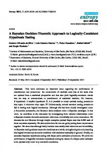
The two previous sections established that statistical view-similarity models can be used to learn the ability to generalize from a single view of previously unseen objects to novel views. In this and subsequent sections, we examine a number of more subtle effects of generalization: dependence on object variability, dependence on training set size, and effects of object classes on the ability to generalize. In the following sections, we are comparing the ability of statistical view-similarity models to generalize under different conditions by comparing the error rates of MLP-based models trained under different conditions using the same training schedule. In these experiments, MLPs are used as a simple learner that contains no particular built-in assumptions or knowledge about visual phenomena like object classes. Of course, we should keep in mind that such experiments with MLPs do not give us definitive answers about the difficulty of a particular problem. But when we find results in such experiments that correlate with psychophysics that demonstrates that very simple learning systems can exhibit seemingly complex view generalization phenomena. That can be an important finding because it raises the question whether we need to devise more complex case-by-case models to explain specific phenomena. Error rates in the following sections are presented as boxplots, as created by the “R” statistical package [17]. These boxplots summarize the error rates from a number (16, unless otherwise noted) of independently trained statistical view similarity MLP models. In such plots, the line at the center of the box represents the median, and the box spans the center two quartiles; points outside the whiskers are considered statistical outliers. Statistical significance of the differences in the medians at the 5% level, where noted, was determined by the “notch” versions of these boxplots, but to avoid cluttering up already complex plots, these are not shown in the paper. For further information on boxplots, the reader is referred to the literature [39].
18
Figure 11: Diagram illustrating the forced choice experiment involving object variability. Under this condition, after their random generation, the vertices of each object are perturbed randomly by Gaussiandistributed vectors. We refer to the standard deviation of these Gaussians as the variability.
10
Object Variability
The above experiments were carried out free of location error and free of object variability: locations were available to the observer with very high accuracy, and in the S = 1 condition, the object giving rise to the two views was geometrically identical–all variation in appearance derived from the differences in viewing parameters. These are common conditions used in experiments in view and appearance based recognition. Real observers face both sensing errors–limitations on the accuracy with which feature locations can be extracted–and object shape variability. We will look here at object variability; the effect of 2D sensing error is very similar for the simple objects we are considering (data not shown). The initial purpose of these experiments was to verify that that the ability to generalize from single views persists in the presence of moderate amounts of sensing error and shape variability. The results themselves also offer some interesting additional insights in the behavior of observers in the presence of error and variability. In these experiments object variability is modeled by displacing each vertex in the 3D model of our paperclip objects independently by a random vector with a Gaussian distribution with covariance matrix diag(σ 2 , σ 2 , σ 2 ). We will refer to σ as the variability. This is illustrated in Figure 11. Figure 12 shows the effect of adding object variability on recognition using 2D similarity. Above a variability of about 0.2, the error rate rises steeply and reaches near chance levels at a variability of about 1.5. To examine the effect of variability on statistical view-similarity models, statistical view-similarity models were trained as before, but all generated training examples (positive and negative) were subject to variability (σL = {0.0, 0.1, 0.2, 0.3}). The resulting networks were then tested under conditions of different amounts of variability (σT = {0.0, 0.1, 0.2, 0.3}). We label experiments conducted with σL and σT as “LσL TσT ”. As before, MLP-based statistical view-similarity models were trained using a collection of 200 objects. All models were trained using the same (unoptimized) learning rate schedule and for the 19
Figure 12: A plot of the error rate using 2D similarity with location features vs. amount of object variability. same number of gradient descent steps (107 ); no overtraining was observed in cross-validation. The results of these experiments are shown in Figure 13. Not surprisingly, the error rate increases with increasing test set variability. There are, in fact, two separate such conditions that are noteworthy. First, we see an increase in error rate keeping the MLP fixed (e.g., L0.0T0.0 through L0.0T0.3). We also see an increase in error rate for the case where the test and training set had the same variability (L0.0T0.0 through L0.3T0.3). We see a decrease in test set error as the training set error approaches the test condition (e.g. L0.0T0.3, L0.1T0.3, L0.2T0.3, L0.3T0.3). Note also that, for example, L0.3T0.0 has a higher rate than L0.0T0.0. Such effects are to be expected in a Bayesian framework: if the training distribution differs from the test distribution, the Bayes optimal solution for the training solution will, in general, not be Bayes optimal for the test distribution. They provide an interesting explanation for what may appear to be otherwise suboptimal human performance: the human perceptual system is optimized for conditions of variability and noise as they occur in the real world; when tested on artificial stimuli exhibiting unusually low variability, a human observer should perform worse, at least initially.
11
Effect of the Number of Training Objects
All experiments reported elsewhere in this paper use views from a random collection of 200 objects as training data for statistical view-similarity models. This has been done in order to demonstrate that even training with a small collection of objects results in the ability to generalize to arbitrary objects. A human subject is likely to bring a lot of prior knowledge about the behavior of vertices under rotation to the task, and may additionally be trained on many more than 200 training samples. It is therefore interesting to see
20
Figure 13: Error rates for training and testing under different conditions of variability. LσL TσT refers to a conditions where training was carried out with variability σL and testing with variability σT . Each boxplot represents the error rates measured for 16 separately trained MLP networks for that condition. Training was on views derived from 200 training objects. Testing was done in 105 trials on 105 novel objects. See the text for a more detailed explanation of the experiment. how much the error rate changes if training is carried out making an arbitrary number of random training objects available to the system. Testing, of course, is still carried out on a separate dataset. Figure 14 shows a comparison of error rates after 106 gradient descent steps for 200 and unlimited numbers of training objects, for object variabilities of 0.0 and 0.1. We see that the performance for unlimited numbers of training objects is somewhat improved relative to the performance of 200 training objects, although the error rates achieved by the best MLP models in each condition are fairly close to one another.
12
Object Classes
Objects that have some geometric similarity but can vary significantly from one another are considered object classes. An object category might comprise passenger cars, faces, planes, or horses. For typical instances of a category, there is some general shape similarity, but the individual variations can be significant and are meaningful. Because objects within a category are geometrically similar to each other, they can be harder to distinguish from one another for an untrained observer compared to distinguishing two arbitrary objects. Such effects have been explored in the psychophysics literature by Tarr [36], Gauthier and Tarr
21
Figure 14: Comparison of error rates for 200 and unlimited numbers of training objects, at variabilities of 0.0 and 0.1. The differences are modest; for a variability of 0.0, the medians are statistically significantly different (p < 0.05). The results show that some variability in results is due to the choice of 200 training objects, but that some residual variability, as well as some outliers, are due to the non-deterministic nature of backpropagation training for MLPs. Each boxplot represents the error rates measured for 16 separately trained MLP networks for that condition. Training was on views derived from 200 training objects. Testing was done in 105 trials on 105 novel objects. [15] and Gauthier et al.[16]. For this paper, we adopt a geometric model of an object category based on a paperclip prototype. Objects within the category are variants, with a given degree of variability as defined above, of the prototype object. Objects outside the category are drawn from the general distribution of random paperclips, as before. This is illustrated in Figure 15. Examples of clips generated under such conditions are shown in Figure 16. Figure 17 shows the behavior of recognition based on 2D similarity for different amounts of variability of category instances relative to a prototype. As expected, if all category instances are very similar to the prototype, it becomes hard to distinguish them based on 2D similarity. Figure 18 shows the performance of statistical view-similarity models on the same task. Condition L0.T0 is learning and testing on general objects. Condition L0.T1 is learning on general objects and testing on in-category objects; because of the greater similarity of in-category objects, the recognition problem is harder and the error rate is considerably higher. Condition L1.T1 consists of learning and testing on incategory objects. The error rate under this condition is statistically significantly lower than under condition L0.T0. These results reproduce some effects observed in psychophysical experiments involving object classes [36]: because of the greater similarity of in-category objects to one another, with only general tranining, the system performs much worse on in-category objects; but once trained on in-category objects, the system 22
Figure 15: Diagram illustrating the forced choice experiment involving object classes. Two objects are derived from a prototype object by displacing the 3D locations of vertices with Gaussian-distributed random vectors of a standard deviation of 0.5 (intraclass variability). Afterwards, the standard forced choice experiment is carried out. Objects not derived from a common prototype are used as a control. In another condition, both objects are subjected to variability after generation from a common prototype. can take advantage of the shape consistency among in-category objects to achieve statistically significantly better performance.
13
Discussion
This paper has presented an approach to learning statistical models of 3D object similarity that generalize to novel, previously unseen object models. The approach, which we refer to as the statistical view-similarity model approach, works by approximating distributions involving two model views and evaluating the similarity of those views in a well-defined probabilistic sense. Relation to Previous Work A significant number of models of view generalization have been proposed, and we have already discussed some of them above. The key difference to the work presented in this paper is that those other models generally assume that multiple training views are available for novel objects, while the work presented in this paper addresses the problem of single view generalization. For example, the linear relationship exploited in [38] (and discussed above) requires at least two novel views. The RBF formulation described in [28] (and also discussed above) also requires multiple training views per object. The same is true for most other models of generalization in 3D object recognition [1, 19, 37, 34]. Any method for single view generalization cannot rely on mathematical relations between multiple known views of the same object, it can only rely on statistical properties of the model base and individual views. That is precisely what is modeled by P (S|x, x0 ) in the above experiments. Since those other models do not perform single view generalization at all, a performance comparison on the single view generalization task is impossible. It might be interesting in future work to compare whether 23
Figure 16: Examples of paperclips used in category-based recognition. single view generalization, applied to multiple sample views, compares comparably to such multi-view generalization methods; this remains to be done for future work. See also the discussion of combination of evidence below. Performance The efficacy of the approach has been demonstrated on a 3D recognition task that has been widely used in machine learning, psychophysics, and neurophysiology: the recognition of 3D paperclips from 2D views, using the same features as used by other authors in previous computational experiments. Using standard methods for estimating conditional probabilities, such as multi-layer perceptrons or empirical distributions (“counting”), this paper has demonstrated up to 20 fold reductions in single-view generalization error rates for novel objects. These reductions in error rates on single-view generalization of completely novel, previously unseen objects were achieved using a training set of only 200 training objects. No retraining or adaptation was required to recognize novel objects, correspondences were not required, and the method did not require explicit maximization of the viewing parameters V prior to recognition. Formulating the single-view generalization problem as that of learning a conditional density P (S|B, B 0 ) or P (B 0 |B, S) is an attractive alternative to interpolation-based or classification-based models of 3D object recognition in the visual system because it addresses a number of issues. The fact that object model acquisition can be carried out almost as easily as storing a new view means that learning of new objects can be very fast and simple; interpolation or classification based methods generally require some kind of parameter adjustment when new objects are added. Furthermore, the fact that integration over the distribution P (V ) of viewing parameters and (in the case of feature maps) correspondence of features between two views is modeled by P (B 0 |B, S) or P (S|B, B 0 ) means that very simple feed-forward networks are sufficient for recognition. In contrast, maximum likelihood methods and other methods that maximize a quality of match function over all viewing parameters are both harder to compute and fail to result in Bayesian optimal decisions in general; a Bayesian optimal procedure must integrate over the unknown 24
Figure 17: A plot of the error rate using 2D similarity in a class-based recognition experiment. The horizontal axis shows the variability among objects within the class. The less in-class objects differ from one another, the harder it is to distinguish them by 2D similarity. viewing parameters, not just maximize over them. Learning from Temporal Continuity Conditional distributions like P (B 0 |B, S) also are easy and natural to learn if we assume some form of temporal continuity: if viewing parameters V = V (t) usuR ally change smoothly with time, then P (B 0 |B, S, θ) = |∆V