Preprints (www.preprints.org) | NOT PEER-REVIEWED | Posted: 1 May 2018
doi:10.20944/preprints201805.0002.v1
Applying Bayesian Network Approach to Determine the Association Between Morphological Features Extracted from Prostate Cancer Images Lal Hussain1*, Sharjil Saeed1, Adnan Idris2, Saeed Arif Shah1, Saima Rathore3, Imtiaz Ahmed Awan1, Sajjad Ahmad Nadeem1 1
Department of CS & IT, The University of Azad Jammu and Kashmir, Muzaffarabad 13100, Azad Kashmir, Pakistan 2 Department of CS & IT, University of Poonch Rawalakot, Rawalakot, Azad Kashmir, Pakistan 3 Department of Radiology, University of Pennsylvania, Philadelphia, PA 19104
Author to whom any Correspondence should be addressed: Corresponding Author: Dr. Lal Hussain Permanent Address: Department of Computer Science & IT, The University of Azad Jammu & Kashmir, Muzaffarabad, 13100, Azad Kashmir, Pakistan E-Mail
[email protected] [email protected]
1
© 2018 by the author(s). Distributed under a Creative Commons CC BY license.
Preprints (www.preprints.org) | NOT PEER-REVIEWED | Posted: 1 May 2018
doi:10.20944/preprints201805.0002.v1
Applying Bayesian Network Approach to Determine the Association Between Morphological Features Extracted from Prostate Cancer Images ABSTRACT - Cancer is a major public health problem across the globe due to which millions of deaths occur every year. In men, Prostate Cancer is estimated as second leading cause of Cancer in the United States. Various factors such as age, family history, diet, sexual behavior and location are mainly involved. Proper and early detection of Prostate Cancer can effectively reduce the mortality rate. In the past researchers extracted multimodal features extracting strategies and employed machine learning and computed aided methods to detect the cancer. However, existing techniques don not provide the detailed individual analysis among the features and strength of relationship for further analysis. In this study, we have proposed Bayesian Network Analysis approach based on morphological features extracted from the Prostate Cancer Imaging Database to determine the relationship between variables and strength of relationship automatically produced by the Network. This analysis will further help that which features are more dominant to establish the relationship and can further increase the detection performance. This approach will be more suitable to find further association among nodes (features). The Mutual Information, Pearson’s Correlation and Kullback Liebler methods were employed to compute the association between the extracted features. The strongest associations are found between variables such as: (Area → Equidiameter), (Area → Circulatory 2), (Circulatory 1→ Entropy), (Circulatory 1→ (Elongatedness), (Circulatory 1→ Max. Radius), and (Min. Radius → Eccentricity). Moreover, node force and impact of interaction among the nodes was also computed. Keywords - Prostate Cancer, Bayesian Network Analysis, Morphological Features, Mutual Information, Pearson’s Correlation and Kullback Liebler
1. Introduction The Prostate Cancer (PCa) in Northern and Western men is commonly diagnosed cancer (>200 per 100 000 men/year) [1] and remain a second leading cause of death in men globally. The projected deaths of Prostate Cancer for 2018 are estimated as 164,690 (19%) and 29,430 (9%) men will die in the United States [2]. In 2018, approximately 609,640 American will die from Cancer corresponding to 1700 deaths per day due to Lung, Prostate, and Colorectum in men and Lung, Breast and Colorectum in women. The PCa is suggested to be the consequence of exogenous factor including chronic inflammation, diet, low exposure to ultraviolet radiation and sexual behaviour [3]. The family history of PCa (both maternal and paternal [4] apart from American African origin, dietary factors, dairy products, body size, sexual behavior and sexually transmitted diseases, smoking, alcohol and age, are the well-established risk factors. The risk increased by 5 to 11 times when two or more first line relatives are affected [5]. About 9% of men suffered from PCa have truly genetic disease associated with an onset of 6-7 years earlier than the spontaneous cases. To analyse the different body parts, Medical imaging has gained much importance within the last few decades [6]. Different clinical diagnostic tools such as prostate specific antigen (PSA), digital rectal examination (DRE), transrectal ultrasound (TRUS) and biopsy tests most widely used for detecting prostate cancer irrespectively of acquiring accurate results [7]. To detect the PCa at early stage, Prostate Specific antigen (PSA) have most extensively been used. It is an imperative to identify new accurate biomarker that allow the early detection of PCa to distinguish aggressive from insignificant tumors. In 2001, about 75% of American men at the age of 50 years or older have undergone to PSA test at least once [8], whereas, this statistics in other countries such as Germany [9] was found lower. In USA, PSA testing is used to detect the prostate cancer in an early phase and has shifted the spectrum of diagnosed cancers towards an increased diagnosis of moderately differentiated tumors. Transrectal Ultrasound-Guided Prostate Biopsy (TRUS-GB) is another tool to evaluate the suspected PCa diagnosis. However, several studies have indicated that TRUS-GB has limitations: having low detection rate of PCa (27-40%), Gleason score underestimation (34-46%) as compare to Gleason score estimated in radical prostatectomy specimens and relatively high detection of clinically insignificant cancers [10–12]. Another promising tool such as Magnetic resonance imaging (MRI) is getting importance to evaluate the PCa. The accuracy 1
Preprints (www.preprints.org) | NOT PEER-REVIEWED | Posted: 1 May 2018
doi:10.20944/preprints201805.0002.v1
for detecting and localizing PCa is improved with the introduction of multiparametric MRI (mpMRI) [13–16]. The research also reveals that use of mpMRI prostate during a magnetic resonance imaging-guided biopsy (MRGB) process has improved the quality of targeted biopsy [17, 18] resulting high detection rate of PCa. In the past researchers extracted various features from MRI images to detect and predict the Prostate Cancer. These features includes texture, morphological, SIFT, EFDs, Local binary patterns (LBP), Gray-level cooccurrence matrix (GLCM), Haar transform and statistical features etc. [19] extracted texture features and obtain a high performance with AUC from 0.81 to 0.85. [20] extracted texture features and applied support vector machine. The cancerous tissues were detected efficiently with high specificity (about 90–95%) and high sensitivity (about 92–96%) by the measurement of the number of correctly classified pixels. Daliri et al. [21] extracted scale-invariant feature transforms (SIFT) features from MRI and classify disease (Alzheimer) using SVM algorithm and got accuracy 86%. Recently [22] extracted texture, morphological, SIFT and EFDs features and applied robust machine learning methods to detect the Prostate cancer. With single features SVM Gaussian kernel give highest accuracy of 98.34% with AUC of 0.999, while using combination of features SVM Gaussian kernel with texture + morphological, and EFDs + morphological features gives highest accuracy of 99.71% and AUC of 1.00. For prognostic and diagnostic of Prostate specimen, different aspects are desired to be considered such as dimension, architectural pattern (poorly formed, cribriform, fused), sector (anterior/ posterior), tumor size, regional part (apex/mild/base), laterality (right/ left) and presence of extra prostatic extension. For proper detection of PCa, geometric features based on morphology are extracted for further analysis. A probabilistic relationship between the variables [23, 24] can be illustrated using Bayesian networks using directed acyclic graphs (DAG). The DAG consists of nodes denoting the clinical variables and edges which connect the nodes represent the conditional dependencies among them. For establishing the network structure for better probabilistic relationship representation between the variables, different approaches and algorithms are used to search the possible networks. Recently, Machine learning has been widely used to analyse the highly complex and multi-dimensional data sets to compute the complicated tasks such as language processing, image processing [25] , or radiological image analysis [26]. These techniques have been rapidly evolving and there is great potential of the applications in clinical neuroscience. In this study, the Bayesian networks using machine learning was employed in which the relationship between the morphological features used in classification [27–29], segmentation [30] etc are extracted from the Prostate Cancer images was established using automated algorithms.
Fig.ure 1. Schematic Diagram of Bayesian Network Analysis Approach based on Morphological Features extracted from Prostate Cancer Images
9
Preprints (www.preprints.org) | NOT PEER-REVIEWED | Posted: 1 May 2018
doi:10.20944/preprints201805.0002.v1
The Fig. 1 shows the schematic diagram of proposed system. In the first step, the images are taken as input from the relevant database. In the second step, the morphological features such as Area, Perimeter, Maximum Radius, Minimum Radius, Elongatedness, Eccentricity, Equidiameter, Entropy, Circulatory 1 and Circulator 2 are extracted from Prostate Cancer Imaging Database. The Bayesian Network analysis approaches are performed for further analysis of the network to determine the strength of relationships between the nodes (morphological features) and significance. .
2. Materials and Methods DATA SET
The Dataset were taken from publicly available database provided by the Harvard University (National Center for Image Guided Therapy Department of Radiology, Brigham and Women Hospital, Harvard Medical School), Harvard medical School and Brigham and woman’s hospital and funded by National Institutes of Health available at (http://prostatemrimagedatabase.com/index.html). The database contains MRI Images for research purposes. In database images are arranged with different series and examination description. In this research, the images of Prostate and Brachytherapy with the last series are taken for further analysis. In the present study, a total of 682 MRIs from 20 patients consisting of 482 images from Prostate subjects and 200 images from Brachytherapy subjects are used for extracting features and employing machine learning classifiers to detect and predict the cancer. FEATURES EXTRACTION
Feature extraction is an important step toward during classification and regression techniques. In the past specific features have been extracted by the researchers for detecting any pathology in the cancer mammograms and other image databases. To detect the colon cancer, . [6, 31, 32] extracted the hybrid and geometric features. .[33] extracted acoustic and Mel frequency cepstral Coefficients (MFCC) features for emotion recognition in human speech, geometric and texture features [34, 35] for detection and recognition of human faces, complexity based features [35, 36] for heart rate variability and to distinguish alcoholic and non-alcoholic subjects. [22] recently extracted texture, morphological, SIFT and EFDs features from Prostate Cancer database and used different machine learning techniques and obtained outer performance result to detect the cancer. The performance obtained using morphological features was also outer performed. The purpose of this study was deeper network relationship analysis using morphological features using node and arc analysis to judge the strength of nodes. MORPHOLOGICAL FEATURES
The morphological tissues are extracted to check whether the tissues are normal or not based on the morphology of the images. These features have been extracted from images by converting the morphology of the images into set of quantitative values for classification tasks [27–29], segmentation [30] and so on. The geometric and shape based features are mostly used to detect the masses present in the medical images [37]. The description of morphological features taken from [38], [39] and implemented in [22]. BAYESIAN NETWORK ANALYSIS
Bayesian networks represent the directed acyclic graphs (DAG) with node and arcs typically cause and effect the relationship between the variables [40]. The Bayesian networks topographic structure reflects the dependency of the variables and illustrate the probability distribution of certain tasks occurred in the specified conditions. Consider X= {X1, X2, X3, ……Xn} a set of m dimensional variables, then the BN is formally defined as a set of couplets =< , > where G denote the DAG in which each node denotes one the variable X1, X2, X3, …. Xn and each arc denote the direct dependency relationship between these variables. Moreover, P denote the set of parameters that quantify the network, contain the probabilities of each possible value xi for each variable Xi. By decomposing the joint probability P under hypothesis that each node is independent of its non-descendants can be computed using joint probability distribution function of the Bayesian Network as: ( )= (
,
,
…….,
)=
(
()
)
Where ( ) denote the set of parent variables of for direct acyclic graph G. The Bayes theorem thus consequently enables to determine the posterior probability through inference of the variable of interest. The variables of interest are extracted as morphological features from Prostate Cancer Database images. The Bayes Networks model analysis was performed using the BayesiaLab V7 software [41] by applying set of supervised 9
Preprints (www.preprints.org) | NOT PEER-REVIEWED | Posted: 1 May 2018
doi:10.20944/preprints201805.0002.v1
learning algorithms to search the optimal model. The information exchanged between target variables and any contaminant was computed using Shannon Entropy [42]. The Shannon Entropy of a discrete variable X is defined as follow: ( )=−
( )
( )
The difference between the condition entropy of the given target (predicted variable) and marginal entropy of the target variable is formally known as Mutual Information [42] and denote by I. Mathematically, the Mutual Information between the variable X and Y is defined by [43] as follow: ( , )=
( )− ( )
Which is equivalent to: ( , )=
( , )
Moreover, conditional Mutual Information (CMI) is defined as: ( , | )=
( , | ) |
( , ) ( ) ( ) ( , | ) ( | ) ( | )
The joint probability distribution of X and Y is denoted by p (X, Y). The marginal distribution of X and Y is represented by p(X) and p (Y) respectively. For data representation in Gaussian distribution [44, 45], the ndimensional Gaussian Distribution with |C| as determinant of covariance matrix of variables X1, X2, X3, …. Xn [46] can be computed as: ( ) = log(2 ) | | By mathematical transforming, the Mi and CMI2 can be computed as follow: | ( )| × | ( )| 1 ( , ) = log | ( , )| 2 CMI2 proposed to integrate interventional probability and Kullback—Leibler divergence [46] to correct the underestimation of CMI [47]. 2( , | ) =
( , , ) , ,
( , )∑
( , , ) ( | , ) ( ) + ( , )∑
( | , ) ( )
CMI2 can be easily computed with the same hypothesis of Gaussian distribution. A complete description and details for computational process with mathematical formulation can be obtained in Zhang’s work [45]. Pearson correlation coefficient (PCC) is a statistical method that measure the direction and strength of a linear relationship between two random variables [48]. PCC has most widely been used in many applications such as data analysis [49], classification [49], decision making and clustering [50], biological research [51], finance analysis [52] etc. The PCC of two variables X and Y is formally defined as the covariance of the two variables divided by the product of their standard deviations [48]. Mathematically: ∑( , ) ∑( , ) = ∑( , ) ∑( , ) denote the mean of X, and = ∑ denote the mean of Y. Where = ∑ The coefficient ranges from -1 to 1and is invariant to linear transformations of either variables. The PCC gives the length of strength of linear relationships between the two random variables X and Y. The positive sign denote that two variables are directly correlated where negative sign denotes that they inversely related. When = 0, then these variables are uncorrelated. When the value of | | is closer to 1, it indicates that there is stronger relationship and closeness to linear relation.
9
Preprints (www.preprints.org) | NOT PEER-REVIEWED | Posted: 1 May 2018
doi:10.20944/preprints201805.0002.v1
3. Results In this study, we extracted ten morphological features from Prostate Cancer imaging database namely Equidiameter, area, Circulatory1, Circulatory2, perimeter, entropy, Elongatedness, max radius, min radius and eccentricity. The arc analysis was performed using Mutual Information (MI), Pearson’s Correlation (PC) and Kullback—Leibler. For node analysis, various factors were considered such as Bayes factor, node force, entropy, mean, normalized mean and reference state probability.
Figure 2. Arc Analysis using Mutual Information (MI) and Kullback – Liebler (KL) Methods
Morphological features are extracted from Prostate Cancer Database Images and Network Relationship Analysis was performed using Mutual Information (MI), Pearson’s Correlation (PC), Kullback- Leibler by arc and node analysis as shown in Fig. 2. The greatest arc strength using MI and KL was obtained 1.0441 between feature pairs (Equidiameter, Area) followed by 0.9154 between the features pair (Circulatory1, Radius), 0.7161 (Circulatory1, Entropy), 0.6804 (Circulatory1, Elongatedness), 0.5275 (Area, Circulatory2), 0.0755 (Min. Radius, Max. Radius), 0.0740 (Circulatory2, Perimeter), 0.0642 (Entropy, Perimeter) and 0.0494 (Min. Radius, Eccentricity).
9
Preprints (www.preprints.org) | NOT PEER-REVIEWED | Posted: 1 May 2018
doi:10.20944/preprints201805.0002.v1
Figure 3. Arc Analysis using Pearson’ s Correlation (PC)
The Arc analysis using PC is depicted in the Fig.3. The greatest Arc Strength was obtained 0.9987 between features pair (Equidiameter, Area) followed by 0.8720 (Min. Radius, Eccentricity), -0.8233 (Circulatory1, Radius), 0.7612 (Area, Circulatory2), -0.7314 (Circulatory1, Elongatedness), 0.7082 (Circulatory1, Entropy), -0.2862 (Circulatory2, Perimeter), -0.2213 (Entropy, Perimeter) and 0.1360 (Min. Radius, Max. Radius).
Figure 4. Node Analysis using Bayes Factor – Arc Analysis using Pearson’s Correlation
9
Preprints (www.preprints.org) | NOT PEER-REVIEWED | Posted: 1 May 2018
doi:10.20944/preprints201805.0002.v1
The network analysis with node (size) using Bayes factor and Arc using PC of Morphological features extracted from Prostate Cancer Images Database is reflected in Fig. 4. The Strengths of Arcs between the adjacent nodes (Morphological features is reflected similarly as show in Fig. 3 of PC.
Figure 5. Network Node Analysis (Node Force) – Arc Analysis using PC
The Greatest Node force was obtained of Circulatory 1 followed by Area, Equidiameter, Max. Radius, Circulatory2, Entropy, Elongatedness and Perimeter as reflected in the Fig. 5. The arc strengths are obtained similar as of PC between each adjacent node.
Figure 6 Network Node analysis using Mean and Arc analysis using PC
The greatest node size is obtained of Perimeter, followed by area, Elongatedness, Equidiameter, Circulatory1, 2, Min and Max. radius, Eccentricity and Entropy as shown in Figure 6.
9
Preprints (www.preprints.org) | NOT PEER-REVIEWED | Posted: 1 May 2018
doi:10.20944/preprints201805.0002.v1
Table 1: Network Performance Analysis with DF of 4
PARENT
CHILD
RW
OC SNMI SRMI GKL % % % TEST 1 25.18 65.87 100.00 994.3664 0.877 22.08 57.76 92.13 871.8372 0.686 17.27 45.18 73.71 682.0175
AREA Equidiameter MAX. RADIUS Circulatory1 CIRCULATORY Entropy 1 CIRCULATORY Elongatedness 0.652 16.41 1 CIRCULATORY Area 0.505 12.72 2 MIN RADIUS Max. Radius 0.072 1.82 PERIMETER Circulatory2 0.071 1.79 ENTROPY Perimeter 0.062 1.55 MIN RADIUS Eccentricity 0.047 1.19
42.93
72.38
648.0441
33.28
48.08
502.3354
4.76 4.67 4.05 3.12
23.74 6.20 5.90 64.89
71.8764 70.522 61.1236 47.052
Legends: RW (Relative Weight), OC (Over all Contribution), SNMI (Symmetric Normalized Mutual Information), SRMI (Symmetric Relative, DF (Degree of Freedom), PC (Pearson’s Correlation)
Based on the different measures, the Bayesian Network showed performance as reflected in above Table. The arc strength between different nodes ( → ℎ ) of KL, MI and PC is reflected in Table and Figures. The highest performance was obtained between nodes ( → ) as KL divergence (1.0441), RW (1), OC (25.18%), MI (1.0441), SNMI (65.87%), SRMI (100%), GKL test (994.3664), P-value (0.00%), PC (0.9987) followed by ( . → 1) as KL (0.9154), RW (0.877), OC (22.08%), MI (0.9154), SNMI (57.76%), SRMI (92.13%), GKL (871.8372), P-value (0.00%), PC (-0.823); ( 1→ ) as KL (0.7161), RW (0.686), OC (17.27%), MI (0.7161), SNMI (45.18%), SRMI (73.71%), GKL (682.0175), P-value (0.00%), PC (0.7082); ( 1→ ) as KL (0.6804), RW (0.652), OC (16.41%), MI (0.6804), SNMI (42.93%), SRMI (72.38%), GKL (648.0441), P-value (0.00%), PC (-0.731); ( 2→ ) as KL (0.5275), RW (0.505), OC (12.72%), MI (0.5275), SNMI (33.28%), SRMI (48.08%), GKL (502.3354), P-value (0.00%), PC (0.7612); ( . → . ) as KL (0.0755), RW (0.072), OC (1.82%), MI (0.0755), SNMI (4.76%), SRMI (23.74%), GKL (71.8764), P-value (0.00%), PC (0.136); ( → 2) as KL (0.074), RW (0.071),OC (1.79%), MI (0.074), SNMI (4.67%), SRMI (6.20%), GKL (70.522),P-value (0.00%), PC (-0.286); ( → ) as KL (0.0642), RW (0.062), OC (1.55%), MI (0.0642), SNMI (4.05%), SRMI (5.90%), GKL (61.1236), P-value (0.00%), PC (-0.221) and ( . → ) as KL (0.0494), RW (0.047), OC (1.19%), MI (0.0494), SNMI (3.12%), SRMI (64.89%), GKL (47.052), P-value (0.00%), PC (0.872).
9
Preprints (www.preprints.org) | NOT PEER-REVIEWED | Posted: 1 May 2018
doi:10.20944/preprints201805.0002.v1
Figure 7. Impact of interaction on the proportion of Morphological features
The variable Perimeter has a mean of 33016.174 and deviation of 1260.157 with probability of 63.41% in the state 0.988. The variable Circulatory 2 has probability of 53.89% of being in the state >0.017, 43.46% in the state of