A Bayesian Game Approach for Intrusion Detection in ... - CiteSeerX

A Bayesian Game Approach for Intrusion Detection in ∗ Wireless Ad Hoc Networks Yu Liu

Cristina Comaniciu

Hong Man

Department of Electrical and Computer Engineering Stevens Institute of Technology Hoboken, NJ 07030, USA



[email protected]

Cristina.Comaniciu@ stevens.edu

[email protected]

ABSTRACT

1.

In wireless ad hoc networks, although defense strategies such as intrusion detection systems (IDSs) can be deployed at each mobile node, significant constraints are imposed in terms of the energy expenditure of such systems. In this paper, we propose a game theoretic framework to analyze the interactions between pairs of attacking/defending nodes using a Bayesian formulation. We study the achievable Nash equilibrium for the attacker/defender game in both static and dynamic scenarios. The dynamic Bayesian game is a more realistic model, since it allows the defender to consistently update his belief on his opponent’s maliciousness as the game evolves. A new Bayesian hybrid detection approach is suggested for the defender, in which a lightweight monitoring system is used to estimate his opponent’s actions, and a heavyweight monitoring system acts as a last resort of defense. We show that the dynamic game produces energy-efficient monitoring strategies for the defender, while improving the overall hybrid detection power.

Ad hoc networks are infrastructure-free, self-organized systems, for which the network operation is based on cooperation of nodes within the neighborhood. In an open environment (i.e. no pre-existing trusted authority), each node agrees to perform network functions such as forwarding and routing. Besides selfishness, ad hoc network misbehavior may be inflicted by malicious nodes, each of which intentionally aims at harming the network operation. A malicious node can mount attacks against different network layers to either compromise individual node(s) or degrade the performance of the overall network. Moreover, existing protocols and techniques for ad hoc networks do not limit end users to use them in a WLAN environment. Hence, if a malicious node can form an ad hoc network with a legitimate WLAN station, it can compromise this station, and then use it as a “backdoor” into the WLAN to stage attacks. Therefore, malicious behavior in ad hoc networks can reach to WLANs and wired networks. IDSs are important means to detect malicious node behavior. In ad hoc networks, most IDSs are proposed to individual nodes (e.g. [1, 2, 3, 4]) due to the lack of centralized management. To better defend a network, every defending node is suggested to be equipped with an IDS, and each IDS is assumed to be always-on. That is to say, each defending node has to be in promiscuous mode. From a system usage perspective, always-on is not an efficient option because mobile nodes are often resource-constrained. To improve defender’s monitoring efficiency, a game-theoretic approach is suggested to model the interactions between attacking node (attacker) and defending node (defender). We formulate the attacker/defender game model in both static and dynamic Bayesian game contexts, and investigate the equilibrium strategies of the two players. The motivation behind our Bayesian game formulation is that generally an attacker/defender game is an incomplete information game [5, p209] where the defender is uncertain about the type of his opponent (regular or malicious). A Bayesian game formulation provides a framework for the defender to select his strategies based on his belief on the type of his opponent. The difference between a static and a dynamic Bayesian game is that the former does not take into account the game evolution, and the defender has fixed prior beliefs about the types of his opponent. In contrast, the latter is a more re-

Categories and Subject Descriptors H.5 [Information Interfaces and Presentation ]: Miscellaneous

General Terms Security, Design

Keywords ad hoc network, noncooperative game, Bayesian game, attacker/defender game ∗This work was supported in part by the ONR grant number N00014-06-1-0063.

Permission to make digital or hard copies of all or part of this work for personal or classroom use is granted without fee provided that copies are not made or distributed for profit or commercial advantage and that copies bear this notice and the full citation on the first page. To copy otherwise, to republish, to post on servers or to redistribute to lists, requires prior specific permission and/or a fee. Valuetools ’06, October 11-13, 2006, Pisa, Italy. Copyright 2006 ACM 1-59593-507-X ...$5.00.

INTRODUCTION

alistic game model, because the defender can dynamically update his beliefs based on new observations of the opponent’s actions and the game history, and then can adjust his monitoring strategy accordingly. In the dynamic game model, a new Bayesian hybrid detection approach is suggested for the defender, with one being used as a lightweight monitoring system to estimate his opponent’s action in each stage game, and the other being used as a heavyweight monitoring system, which functions as a last resort of defense. The heavyweight monitoring system is assumed to have more detection power than the lightweight monitoring system, e.g., can resolve attack sources or has higher detection rate. We show that the dynamic game produces energy-efficient monitoring strategies for the defender, while improving the overall hybrid detection power. The rest of the paper is organized as follows. Section 2 introduces the static Bayesian game model, and Bayesian Nash equilibrium solutions are investigated. Section 3 describes the dynamic Bayesian game model, and perfect Bayesian equilibrium solutions are studied. Section 4 considers multiplayer scenarios for both game models. Section 5 presents numerical examples for the proposed games. Section 6 discusses related work. Finally, Section 7 concludes the paper.

2. 2.1

since otherwise the attacker does not have incentive to attack and the defender does not have incentive to monitor. In a resource-constrained network, cost of monitoring (cm ) can be defined as a function of energy consumption with respect to the monitoring activities; cost of attacking (ca ) can be defined as a function of energy consumption with respect to the attack activities. Table 1: Strategic form of static Bayesian game

Attack Not attack

Monitor (1 − 2α)w − ca , (2α − 1)w − cm 0, −βw − cm

Not monitor w − ca , −w 0, 0

(a) Player i is malicious

Not attack

Monitor 0, −βw − cm

Not monitor

0, 0

(b) Player i is regular

STATIC BAYESIAN GAME Game Model

Consider a flat ad hoc network with a fixed number of N nodes in the network. It is assumed that any defending node is equipped with an IDS. Depending on the capability of the IDS, the defending node can detect an attacking node in the neighborhood or any node in the network. We consider a two-player static Bayesian game. One player is a potential attacking node, denoted by i. The other player is a defending node, denoted by j. Player i has private information about his type, which is either regular, denoted by θi = 0, or malicious, denoted by θi = 1. In other words, the maliciousness of player i is unknown to defender j. Defender j is of regular type denoted by θj = 0. The type of defender j is common knowledge to the two players. The malicious type of player i has two pure strategies: Attack and Not attack. The regular type of player i has one pure strategy: Not attack. Defender j has two pure strategies: Monitor and Not monitor. The two players choose their strategies simultaneously at the beginning of the game, assuming common knowledge about the game (costs and beliefs). Assume defender j’s security value is worth of w, where w > 0. In practice, w could be the (monetary) value of protected assets. In other words, −w represents a loss of security whose value is equivalent to a degree of damage such as loss of reputation, loss of data integrity, cost of damage control, etc. Therefore w is subject to different security policies. We also assume that there is an equal gain/loss w for both the defender and the attacker. This is reasonable when dealing with malicious nodes (as opposed to selfish nodes). Table 1 illustrates the payoff matrix of the game in strategic form. In the matrix, α represents the detection rate (i.e. true positive rate) of the IDS, β represents the false alarm rate (i.e. false positive rate) of the IDS, and α, β ∈ [0, 1]. w is defender j’s security value. Costs of attacking and monitoring are denoted by ca and cm respectively, where ca , cm > 0. It is reasonable to assume that w > ca , cm ,

In Table 2(a), for the strategy combination (Attack, Not monitor ), defender j’s payoff is −w, and the malicious type of player i’s payoff is his gain of success minus the attacking cost, i.e. w − ca . For the strategy combination (Attack, Monitor ), defender j’s payoff is the expected gain of detecting the attack minus the monitoring cost cm . The expected gain of detecting the attack depends on the value of α, which is αw − (1 − α)w = (2α − 1)w. Note that 1 − α is the false negative rate. In contrast, the malicious type of player i’s gain is the loss of defender j, which is (1 − 2α)w. Thus the payoff of player i is his gain minus the attacking cost. For the other two strategy combinations, when player i plays Not attack, his payoff is always 0. In both cases, defender j’s payoff is 0 if he decides not to monitor, and he has a monitoring cost cm and an expected loss −βw due to false alarms if he monitors. In Table 2(b), the payoff of the regular type of player i is always 0. The payoff of defender j is 0 if he decides not to monitor, and has a monitoring cost cm and an expected loss due to the false alarm, −βw, if he monitors.

2.2

Bayesian Nash Equilibrium (BNE) Analysis

Suppose defender j assigns a prior probability µ0 to player i being malicious. Figure 1 illustrates the extensive form of the static Bayesian game. In the figure, node N represents a “nature” node, who determines the type of player i. The objective of both players is to maximize their expected payoffs. This implies that we assume that both players are rational. This assumption is a generic assumption for a well-defined game, and it fits in perfectly with the attackerdefender scenario in the sense that the attacker would like to play a Bayesian strategy to minimize his chances of being detected, and the defender would also want to play a Bayesian strategy in order to maximize his chance of detecting attacks without overspending his energy on monitoring. Adopting a non-Bayesian strategy is expected to reduce the players’

By imposing Euj (Monitor ) = Euj (Not monitor ), we get that the malicious type of player i’s equilibrium βw+cm . strategy is to play Attack with probability p∗ = (2α+β)wµ 0 Similarly, By imposing Eui (Attack ) = Eui (Not attack ), we get that defender j’s equilibrium strategy is to play a Monitor with probability q ∗ = w−c . Thus, strategy 2αw ∗ pair ((p if malicious, Not attack if regular), q ∗ , µ0 ) is a mixed-strategy BNE.

Figure 1: Extensive form of static Bayesian game payoffs. In the following, we analyze BNE based on the assumption that µ0 is a common prior, i.e. player i knows defender j’s belief of µ0 . • If player i plays his pure strategy pair (Attack if malicious, Not attack if regular), then the expected payoff of defender j playing his pure strategy Monitor is Euj (Monitor ) = µ0 ((2α−1)w−cm )−(1−µ0 )(βw+cm ), and his expected payoff of playing his pure strategy Not monitor is Euj (Not monitor ) = −µ0 w. So if Euj (Monitor ) > Euj (Not monitor ), or if µ0 > (1+β)w+cm , then the best response of player j is to (2α+β−1)w play Monitor. However, if defender j plays Monitor, Attack will not be the best response for the malicious type of player i, and he will move on to play Not attack instead. Hence, ((Attack if malicious, Not attack if regular), Monitor, µ0 ) is not a BNE. However, if m µ0 < (1+β)w+c , the best response for defender j is (2α+β−1)w Not monitor and thus ((Attack if malicious, Not attack if regular), Not monitor, µ0 ) is a pure-strategy BNE. • If the malicious type of player i plays his pure strategy Not attack, defender j’s dominant strategy is to play Not monitor, regardless of µ0 . However, if defender j plays Not monitor, the best response for the malicious type of player i is to play Attack, which reduces to the previous case. So strategy ((Not attack if malicious, Not attack if regular), Not monitor ) is not a BNE. • We previously showed that no pure-strategy BNE exm ists for the game when µ0 > (1+β)w+c . A mixed(2α+β−1)w strategy BNE is derived as follows. Let p be the probability with which player i plays Attack, and q be the probability with which defender j plays Monitor. The expected payoff of defender j playing Monitor is Euj (Monitor ) =pµ0 ((2α − 1)w − cm ) − (1 − p)µ0 (βw + cm ) − (1 − µ0 )(βw + cm ), and the expected payoff of defender j playing Not monitor is Euj (Not monitor ) = −pµ0 w.

In summary, the static Bayesian game has no pure-strategy m , but has a mixed-strategy BNE ((p∗ BNE if µ0 > (1+β)w+c (2α+β−1)w if malicious, Not attack if regular), q ∗ , µ0 ). That is, if defender j’s belief about the maliciousness of player i is high m enough (µ0 > (1+β)w+c ), a mixed-strategy BNE exists for (2α+β−1)w which defender j plays Monitor with probability q ∗ , and player i plays Attack with probability p∗ if malicious and plays Not attack if regular. We also see that if defender j’s belief about the maliciousness of player i is very low m (µ0 < (1+β)w+c ), a pure-strategy BNE ((Attack if mali(2α+β−1)w cious, Not attack if regular), Not monitor, µ0 ) exists. That is, a pure-strategy BNE exists for which defender j plays his pure strategy Not monitor, and player i plays his pure strategy Attack if malicious and Not attack if regular. Note that the static Bayesian game model is general enough to model most types of attacks in ad hoc networks provided that the IDS is designed to handle these types of attacks. Examples of these kind of attacks supported by the Bayesian model include denial-of-service (DoS) attacks at different network layers (e.g., network layer and transport layer), routing disruption attacks at the network layer, etc. The only exception, is that the Bayesian framework cannot model defense for colluding attacks, due to the game assumption that every node’s action is independent of other nodes’ actions. The advantage of using a static Bayesian game model is that instead of applying an always-on IDS monitoring strategy, the defender can implement an efficient monitoring strategy according to his BNE solution that maximizes his expected payoff. One possible drawback in practice is that it may be hard to determine a reasonable prior probability µ0 . In practical applications, the defender can assign µ0 based on his knowledge of the network environment: if it is a hostile environment, a high value of µ0 can be assigned.

3.

DYNAMIC BAYESIAN GAME

The aforesaid static Bayesian game is a one-stage game, for which the defender maximizes his payoff based on a fixed prior belief about the maliciousness of his opponent. Due to the difficulty of assigning accurate prior probabilities for player i’s types, we extend the static Bayesian game to a multi-stage dynamic Bayesian game, where the defender updates his beliefs according to the game evolution. We assume that the static Bayesian game is repeatedly played in each time period tk , where k = 0, 1, .... An interval of T seconds may be selected for each stage game. We consider that the game has an infinite horizon because in general any node will not have the information about when his neighboring node leaves the network. The payoffs of the players in each stage game are the same as in the preceding static game, and we assume that there is no discount factor with respect to the payoffs of the players. That is to say that the payoffs remain the same in every stage

game. Furthermore, we assume that the players’ identities remain consistent throughout the game. This implies that the proposed dynamic game model relies on authentication mechanisms to counteract spoofing, impersonation, and the Sybil [6] attacks. An example of authentication protocol for ad hoc networks is TIK, proposed by Hu et al. in [7]. Continuing with the notations presented in the preceding static game, a potential attacker is denoted by i, and a defender is denoted by j. Player i’s type θi is private information. Defender j’s type is regular (θj = 0), and it is common knowledge. The players choose actions simultaneously at the beginning of each stage game. The extensive form of each stage game can be represented in a similar manner as for the static Bayesian game (see Figure 1). We suppose in the beginning of each stage game tk , the malicious type of player i chooses an action ai (tk ) in Ai = {Attack, Not attack }, or the regular type of player i chooses his only action Not attack ; defender j chooses an action aj (tk ) in Aj = {Monitor, Not monitor }. Similar to the static game, we can define mixed strategies for the constituent static games. For dynamic game, these mixed strategies depend on the history of the game and are denoted as behavior strategies. A behavior strategy specifies a probability distribution over actions at each information set. Specifically, a behavior strategy for player i, denoted by σi , is defined as σi (ai (tk )|θi , hji (tk )), where hji (tk ) represents the action history profile of player i with respect to his opponent j at the beginning of stage game tk . We define a behavior strategy for defender j as σj (aj (tk )|θj , hij (tk )), where hij (tk ) represents the action history profile of defender j with respect to his opponent i at the beginning of stage game tk . We define the action history profile of player i with respect to defender j at stage game tk , hji (tk ), as a binary vector that contains actions of player i at each stage game t0 , ..., tk−1 , which is hji (tk ) = (aji (t0 ), ..., aji (tk−1 )),

(1)

aji (tk )

where indicates player i’s action with respect to defender j at stage game tk . In what follows, to simplify the exposition, we will use an abuse of notation and denote

game tk to tk+1 using Bayes’ rule. Specifically, defender j updates his beliefs about the types of his opponent i at the end of each stage game by calculating his posterior beliefs, defined as µj (θi |ai (tk ), hji (tk )), where ai (tk ) represents player i’s action at stage game tk , and hji (tk ) represents the action history profile of player i with respect to defender j. From Bayes’ rule, the posterior beliefs of player j can be computed as follows: µj (θi |ai (tk ), hji (tk )) µj (θi |hji (tk ))P (ai (tk )|θi , hji (tk )) , = P ˜ j ˜ j θ˜i µj (θi |hi (tk ))P (ai (tk )|θi , hi (tk ))

(2)

where µj (θ˜i |hji (tk )) > 0, hji (tk ) > 0, and P (ai (tk )|θi , hji (tk )) is the probability that action ai is observed at this stage of the game, given the type of the opponent and the history of the game. From Equation (2), we see that, in order to update the belief, at stage game tk , defender j first needs to “observe” i’s action ai (tk ). From defender j’s point of view, the action (Attack or Not attack ) of player i at each stage game can be observed (detected) by an always-on monitoring system. As described in the preceding static game model, always-on monitoring is not an energy-efficient strategy, instead the defender can use the static game model to derive a better solution. However, although each stage game is considered as a static Bayesian game, this solution will not fit in the stage games of the dynamic model, because belief updating requires the defender to constantly observe the actions of his opponent at each stage game. To save the energy spent on the IDS, we propose a Bayesian hybrid detection approach that comprises of two monitoring systems: lightweight monitoring system and heavyweight monitoring system. The assumption is that the latter is a more sophisticated IDS which provides more detection power, but consumes more energy. The objective of the hybrid detection approach is to derive efficient monitoring strategies for the two monitoring systems based on a dynamic Bayesian game formulation.

3.2

Bayesian Hybrid Detection

σi (ai (tk ) = Attack|θi , hji (tk )) = p, σi (ai (tk ) = Not attack|θi , hji (tk )) = 1 − p, σj (aj (tk ) = Monitor|θj , hij (tk )) = q, and

History Profile

σj (aj (tk ) = Not monitor|θj , hij (tk )) = 1 − q, with the understanding that the mixed strategies p and q for a stage game, will depend on the current information set of the game (the history of the game). In a stage game tk , defender j’s optimal behavior strategy, depends on his beliefs about the types of player i at the beginning of tk . In the first stage game t0 , defender j’s belief of player i being malicious is characterized by a prior probability µ0 . In the subsequent stages of the dynamic game, defender j can update his beliefs at the end of each stage game based on his observed action of player i and the action history profile of the game.

3.1

Bayesian Updating Rule for Beliefs

We construct a belief updating system for defender j, so that the beliefs of defender j can be updated from stage

Belief Updating System

No

Lightweight IDS

Audit Data Input

Heavy Monitoring?

Yes

Heavyweight IDS

Audit Data Input

Detection Output

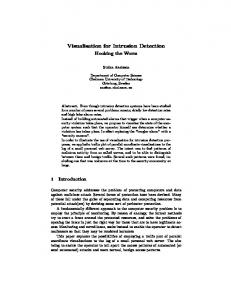
Figure 2: The Bayesian hybrid detection framework. Figure 2 illustrates the framework of the proposed Bayesian hybrid detection approach. As shown, the decision on setting on or off the heavyweight IDS depends on the output of the belief updating system, which in turn utilizes the information from the lightweight monitoring system and the game history profile as the inputs. In other words, the defender decides whether to activate the heavyweight monitoring system in next stage game based on his updated beliefs

of the types of player i at the end of current stage game. The output of the heavyweight IDS can update (or reset) the defender’s belief. Note that once the heavyweight IDS is on, the lightweight monitoring is off, so that only one system is active at a time. To realize the proposed Bayesian hybrid detection approach in practice, we suggest one heavyweight system as the last-resort IDS. We then suggest two lightweight monitoring systems, with one emphasizing on detecting maliciousness of the entire neighborhood (i.e., player i, the defender’s opponent, is the entire neighborhood instead of a single node), and the other emphasizing on evaluating neighboring nodes individually (i.e., pairwise attacking/defending node interactions are monitored). 1) One heavyweight monitoring system For the heavyweight monitoring system, we consider an anomaly based IDS which we previously proposed in [8]. This system employs an association-rule mining technique to find association patterns from a set of packet-level transaction events, which consist of features collected according to Table 2. The IDS builds a normal profile by extracting association rules from training data. Association rules extracted from test data are then compared against the normal profile. Any deviance from the norm is considered as an anomaly rule, which may trigger an intrusion alert accordingly. Table 2: Cross-layer feature set Dimension Flow direction (Dir) Send address (SA) Destination address (DA) MACFrameType RtPktType*

Value Space SEND, RECV, DROP sai , ∀i ∈ node set S daj , ∀j ∈ node set S RTS, CTS, DATA, ACK RtDataPkt, RtCtrlPkt

*This feature dimension applies to MAC DATA frame only.

The advantage of this IDS is the ability to identify attack source(s) within one-hop perimeter due to the use of MAC addresses as features for intrusion detection. However, the size of audit data collected from the MAC layer traffic is usually large even for a short time interval. Thus, the normal profile usually contains a large set of rules, even if some aggregation and pruning steps are taken. 2) Two lightweight monitoring systems Cross-feature analysis system The cross-feature analysis system is an anomaly detection system that employs the cross-feature mining technique proposed by Huang et al. [9]. This technique explores intercorrelations among features in a feature vector. The details of this system are presented in [10]. Briefly, the cross-feature mining technique is applied to data collected on statistical features, as specified in Table 3. The feature set is defined on the MAC layer data (assume 802.11 MAC), so that the monitoring range of the system is within the neighborhood. A feature vector f = {f1 , f2 , ..., fk } is a set of quantized feature values collected according to Table 3. Given a feature vector f = {f1 , f2 , ..., fk } in a data set, the inter-correlation value of fi , denoted by ri , with respect to f is defined as the conditional probability of fi . That is, ri = pi (fi |f1 , f2 , ..., fi−1 , fi+1 , ..., fk ). An overall P interr correlation value of f, denoted by R, is defined as R = ki i .

If R > θ, where θ is a decision threshold, f is classified as a normal feature vector. A normal profile consists of a set of normal feature vectors constructed from training data. For test data, each constructed feature vector is tested against the normal profile, and any deviance may trigger an intrusion alert. Table 3: Statistical feature set Feature Time Network allocator value Transmit traffic rate Receive traffic rate Retransmit RTS Retransmit DATA Neighbor node count Forwarding node count

Value Space ignored in classification continuous continuous continuous discrete discrete discrete discrete

Unit second second byte byte count count count count

The advantage of this IDS is that the audit data size is dramatically smaller than the one used in the associationrule anomaly detection system. Thus, less time would be spent on both training and testing. Nevertheless, the inclusion of the latter can help to identify the attack source(s). Note that the cross-feature analysis system is unable to provide attack source information, thus, in the game model, player i represents the entire neighborhood of defender j. To use the cross-feature analysis system in the dynamic Bayesian game, we consider each sampling interval of the cross-feature analysis system, e.g. 5 seconds, as the time period of a stage game. The action of Attack is determined when the feature vector is classified as an abnormal feature vector, and in contrast, the action of Not attack is determined when the feature vector is classified as a normal feature vector. Following the determination of player i’s action, defender j updates his beliefs about the types of player i. In the next stage game, whether the association-rule analysis (heavyweight monitoring) is activated or not, depends on defender j’s posterior belief about player i being malicious, and on the costs associated with each action, according to the game formulation. Coarse-grained node-to-node analysis system If interested in evaluating neighboring nodes individually, pairwise attacking/defending node interactions need to be monitored. Because association-rule analysis is not suitable for always-on monitoring due to the massive packet-level transactions in MAC layer and network layer, we propose the following lightweight monitoring system to substitute the cross-feature analysis so that the beliefs of defender i can be updated consistently on consecutive stage games. Let Γj denote the set of neighboring nodes of defender j, where Γj ∈ N . We consider that a potential attacker i is a neighbor of j, so i ∈ Γj . We assume i and j have symmetric links, thus j ∈ Γi . We denote Rji (tk ) as the number of packets received at node j from node i. The normalized reception ratio (NRR) of node j from node i for stage game tk , denoted by ψji (tk ), is given by Rji (tk ) v∈Γj u6=v Ru∈Γj (tk ) +

ψji (tk ) = P

v∈Γj

Rj

(tk )

.

(3)

So, NRR of node j reflects the level of inbound traffic

rate at node j from node i with respect to the overall traffic rate of the neighborhood of node j. The Attack action of player i is determined by applying threshold value τ , where τ is considered as a caution level of node j with respect to player i. That is, ai (tk ) = Attack, if ψji (tk ) > τ.

(4)

From Equations (3) and (4), we see that the complexity of the coarse-grained node-to-node (attacker-to-defender) analysis system is much less than that of the association-rule analysis system which we use it as the heavyweight IDS. In addition, from Table 2, we see that the association-rule analysis includes multiple features (5 feature dimensions and at least 24 features without considering the number of active nodes in the network) for anomaly detection. On the other hand, the coarse-grained node-to-node analysis system only uses one NRR feature. Furthermore, in the association-rule analysis, a normal file usually consists of tens to hundreds association rules. This means that each rule extracted from test data needs to be compared against all the rules in the normal profile. In contrast, the coarse-grained node-to-node analysis system requires only one one comparison at each stage game to determine the action of player i. The choice of τ influences the performance of coarse-grained node-to-node analysis. Although τ may be determined experimentally by learning the normal traffic pattern in the network, its accuracy is limited by the bursty nature of data traffic. Nonetheless, in our previous work [8], we have shown that using this simple traffic analysis as a preprocessing step for the association-rule analysis leads to a lower false positive rate for the overall system. The drawback of the coarsegrained node-to-node analysis system is that it can only detect inbound traffic attacks such as sleep deprivation, flooding, and some DoS attacks, and it misses outbound traffic attacks such as blackhole and packet dropping attacks.

3.3

Belief Updating in the Presence of Observation Errors

Since the lightweight monitoring system may inevitably produce false positives and false negatives, the “observed” actions may not always accurately reflect the reality. We incorporate the effect of false alarm and misdetection errors for the lightweight IDS, in updating the beliefs by appropriately determining the conditional probabilities P (ai (tk )|θi , hji (tk )). More specifically, denoting with αp and βp the detection rate and false positive rate of the lightweight monitoring system, respectively, the above conditional probabilities can be updated as follows: P (ai (tk ) = Attack|θi = 1, hji (tk )) = αp × p + βp × (1 − p),

(5)

and P (ai (tk ) = Not attack|θi = 1, hji (tk )) = (1 − αp ) × p + (1 − βp ) × (1 − p),

(6)

and P (ai (tk ) = Attack|θi = 0, hji (tk )) = βp ,

(7)

P (ai (tk ) = Not attack|θi = 0, hji (tk )) = 1 − βp .

(8)

and

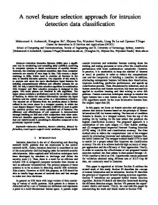
Note that 1 − αp represent the false negative rate, and 1 − βp represent the true negative rate. We used the notations αp and βp in Equations (5)-(8) to differentiate from the detection rate α and the false positive rate β defined in the payoff functions of defender j, which refer to the heavyweight monitoring system. Provided that defender j can determine player i’s action and behavior strategy in each stage game according to the preceding subsections 3.2 and 3.3, defender j can then update his beliefs about the types of player i using Equation (2). Figure 3 demonstrates the convergence of defender j’s posterior beliefs under various αp , βp , and cwa . Figures 3(a) and (b) assume the parameters in the payoff functions of the defender are: α = 0.9, β = 0.01, cwm = 1000 and cwa = 1000, and Figure 3(c) assumes α = 0.9, β = 0.01, αp = 0.8, βp = 0.01. For all three scenarios, defender’s prior probability µ0 = 12 . From Figure 3(a), we see that the higher αp is, the faster posterior belief converges to 1. By contrast, Figure 3(b) shows that the lower βp is, the faster posterior belief converges to 1. In other words, the convergence speed of defender j’s posterior belief increases with the detection accuracy of the lightweight monitoring system. From Figure 3(c), we see that the higher the ratio of security value w to the attacking cost ca is, the faster the convergence speed of defender j’s posterior beliefs will be. The ratio of w versus monitoring cost cm influences the convergence speed in a similar manner.

3.4

Perfect Bayesian Equilibrium (PBE) Analysis

A Dynamic Bayesian game is a multi-stage game with observed actions and incomplete information. In a sequential game, the players best responses are often guided by the threats about certain reactions for other players. For a sequential game with incomplete information, such threats are dependent on the current beliefs, which may change as the game evolves. The concept of PBE defines the proper interaction between users’ beliefs about types, given a selection of actions, and the actual strategies. PBE requires that players form a complete system of beliefs about the opponents’ types at each decision node that can be reached, update this beliefs according to a Bayes’ rule, and the take best response actions using regular Bayesian Nash equilibrium. PBE demands that subsequent play should be optimal for every stage of the game, i.e., it is related to the concept of subgame perfection. In what follows, we show that our proposed multi-stage attacker/defender game has a PBE. We first show that the proposed multi-stage attacker/defender game satisfies the Bayesian conditions B(i)-B(iv) and equilibrium condition P. The above conditions guarantee that the incomplete-information game has a PBE [5, p333]. Lemma 1: The described multi-stage attacker/defender game satisfies the four Bayesian conditions B(i)-B(iv): B(i) Posterior beliefs are independent, and all types of player j have the same beliefs, and even unexpected events will not change the independence assumption for the type of the opponents. B(ii) Bayes’ rule is used to update beliefs from µj (θi |hji (tk )) to µj (θi |hji (tk+1 )) whenever possible. B(iii) The players do not signal what they do not know. B(iv) All players must have the same belief about the type

1

Posterior belief of defender µj(θi = 1|"Attack")

0.95

0.9

0.85

0.8

0.75

0.7

0.65

0.6

α = .5 p αp = .7 α = .9

0.55

p

0.5

0

5

10

15

20

25

30

Number of stage games k

(a)

of another player. The proof of Lemma 1 is rather trivial because this is a two-player game. Briefly, B(i) is trivially satisfied because defender j has only one type. From the proposed belief updating system, we see that the game satisfied B(ii). Condition B(iii) means µj (θi = 1|(ai (tk ), hji (tk ))) = µj (θi = 1|(b ai (tk ), hji (tk ))), if ai (tk ) = b ai (tk )). In our attack/defender game context, attacker’s signal is part of attack actions, thus B(iii) is satisfied. For condition B(iv), because at any stage game only two players are in the game, and there are no other players influencing the belief updates of the two players. In essence, Lemma 1 states that each player’s belief updating is consistent in every stage game. Based on the assumption of rationality of players, at each stage game, defender j’s optimal strategy is to maximize his payoff according to his new beliefs. Definition 1: In the described multi-stage attacker/defender game, defender j’s optimal behavior strategy σj∗ with respect to his beliefs about player i’s type µj (θi |ai (tk ), hji (tk )) at stage game tk satisfies the following relation:

1


0.95

0.9

0.85

0.8

0.75

0.7

0.65

0.6

β = .001 p βp = .01 β = .05

0.55

p

0.5

0

5

10

15

20

25

30


(b) 1

ui ((σi∗ , σj )|θi , hij (tk ), µi (·)) ≥ ui ((σi0 , σj )|θi , hij (tk ), µi (·)), (10) where σi0 is an alternative behavior strategy of i, and hij (tk ) is the action history profile of j with respect to i, µi (·) is the abbreviation of µi (θj |aj (tk ), hij (tk )), and ui (·) is player i’s expected payoff under strategy profile (σi∗ , σj ) at stage game tk . Since j has only one type, Equation (10) reduces to

0.95


uj ((σi , σj∗ )|θj , hji (tk ), µj (·)) ≥ uj ((σi , σj0 )|θj , hji (tk ), µj (·)), (9) where σj0 is an alternative behavior strategy of defender j, and hji (tk ) is the action history profile of player i with respect to defender j, µj (·) is the abbreviation of µj (θi |ai (tk ), hji (tk )), and uj (·) is the expected payoff of defender j under strategy profile (σi , σj∗ ) at stage game tk . Analogously, we define potential attacker i’s optimal strategy as follows. Definition 2: In the described multi-stage attacker/defender game, the optimal behavior strategy of a potential attacker i, denoted by σi∗ , with respect to his beliefs µi (θj |aj (tk ), hij (tk )) at stage game tk satisfies the following condition:

0.9

0.85

0.8

0.75

0.7

0.65

0.6

0.5

ui ((σi∗ , σj )|θi , hij (tk )) ≥ ui ((σi0 , σj )|θi , hij (tk )).

w/c = 10 a w/c = 100 a w/c = 1000 a

0.55

0

5

10

15

20

25

30


(c) Figure 3: Convergence of defender’s posterior beliefs given the observations of a sequence of consecutive Attack actions (a) under various αp , (b) under various βp , (c) under various ratios of w/ca .

(11)

Lemma 2: The described multi-stage attacker/defender game satisfies the equilibrium condition P for multi-stage games of incomplete-information: (P) For each player x, type θx , player x’s alternative strategy σx0 , and history h(tk ), the expected payoff achieved by employing strategy σx , denoted by ux , satisfies the following condition: ux (σ|h(tk ), θx , µ(·|h(tk ))) ≥ ux ((σx0 , σ−x )|h(tk ), θx , µ(·|h(tk ))).

(12)

In essence, condition P states that each player’s behavior strategy is sequential rational in each stage game. By Definitions 1 and 2, given defender j’s belief µj , the multi-stage

attacker/defender game has a strategy pair σ = (σi∗ , σj∗ ) that satisfies the above inequality formula, hence condition P is satisfied. Theorem 1: The described multi-stage attacker/defender game has a perfect Bayesian equilibrium. Proof: Since the described multi-stage attacker/defender game satisfies the four Bayesian conditions B(i)-B(iv) (Lemma 1) and the equilibrium condition P (Lemma 2), the game has a strategy profile (σ, µ), where σ = (σi∗ , σj∗ ) is a strategy pair for the two players, and µ = (µi (θj |hij (tk )), µj (θi |hji (tk ))) is the vector of beliefs for the two players. Note that µi is not needed since θj ’s type is common knowledge. By the definition of PBE [5, p333], (σ, µ) is a PBE. In the subsequent paragraphs, we determine the PBE for each stage game. We analyze the dynamic game as a Bayesian signaling game, in which the actions of potential attacker i signal his type to defender j. Due to the fact that defender j relies on an always-on monitoring system (crossfeature analysis system or lightweight monitoring system) to determine the actions of his opponent i, which is not error free, the equilibrium we seek is always a semi-separating equilibrium. Note that the other two possible equilibria for signaling games, separating and pooling equilibria, do not apply for our scenario [5]. The separating case occurs if the type of the potential attacker i can be perfectly determined after signaling, while in the pooling case, the two types of i cannot be distinguished based on their behavior. The semi-separating equilibrium, is given by the strategies that maximize both players’ payoffs, while none of the players have an incentive to change its strategy. We can see that only a mixed strategy equilibrium exists for each stage game. To determine this mixed strategy equilibrium we rely on the indifference condition for players’ different strategies. At stage game tk , if defender j observes that the action of his opponent i was Attack, then his expected payoff for playing Monitor is Euj (aj (tk ) = Monitor |ai (tk ) = Attack ) = (((2α − 1)w − cm )p + (−βw − cm )(1 − p))µj (θi = 1|·) + (−βw − cm )µj (θi = 0|·), (13) and his expected payoff for playing Not monitor conditional on his observation is Euj (aj (tk ) = Not Monitor |ai (tk ) = Attack ) = −wpµj (θi = 1|·).

(14)

So, player i chooses p∗ (the probability with which player i plays Attack ) to keep defender j indifferent between Monitor and Not monitor. That is, p∗ is derived by setting Equations (13) and (14) equal. Consequently, we have p∗ =

βw + cm . (2α + β)wµj (θi = 1|·)

w − ca . (17) 2αw The PBE for the game is given as (p∗ , q ∗ , µ(.)), with p∗ , ∗ q , µ(.)) given by Equations (15), (17), and (2), respectively. To see why there is no pure strategy equilibrium for this game, we determine the best response strategy (BR) for both players to be q∗ =

BRj = Monitor if p >

βw + cm , (2α + β)wµj (θi = 1|·)

(18)

w − ca . (19) 2αw If (18) holds ⇒ monitor, q = 1 ⇒ (19) does not hold ⇒ not attack, p = 0 ⇒ (18) does not hold ⇒ not monitor, q = 0, ... Using the above argument, we see that there is no pure strategy equilibrium for the analyzed dynamic Bayesian game. BRi = Attack if q
0, since Ej > ej . Besides saving energy consumption cost, the use of hybrid detection framework can also reduce the probability of false alarm for the overall equivalent IDS. Our simulation results show that by adding the very simple coarse-grained node-to-node analysis system in front of the association-rule analysis system will reduce the probability of false alarm for the overall equivalent IDS.

(15)

On the other hand, q ∗ (the probability with which defender j plays Monitor ) is selected to keep the malicious type of player i indifferent between his strategies Attack and Not attack. The indifference condition is given as (((1 − 2α)w − ca )q + (w − ca )(1 − q)) = 0,

and thus defender j’s equilibrium strategy is to choose q ∗ as

(16)

4. MULTIPLAYER CONSIDERATION Both the static and dynamic Bayesian games proposed so far, are two-player games. As we have already mentioned for the cross-feature analysis IDS, the two-player game can also be set up as the defender, against his entire neighborhood. This relaxes the assumption of pairwise interactions in the attacker/defender game.

Overall inter−correlation probability of feature vector (%)

0.6 0.5 0.4 0.3 normal

θ = 0.2

0.2 abnormal

0.1 0

0

5

10

15

20

25

30

20

25

30

0.7 0.6 0.5 0.4 0.3 normal

θ = 0.2

0.2 abnormal

0.1 0

0

5

10

15

Sampling data points (5s/point)

(a) 1

0.9

j

i

Posterior belief of defender µ (θ = 1| ⋅)

In this section, we provide examples to illustrate the equilibrium achieved for the dynamic Bayesian game. We use the cross-feature analysis to determine actions of a potential attacker in each stage game. In our previous work [8, 10], we have simulated a network of 500 x 500 square meters on the network simulator ns2 [11] platform, and evaluated the performance of the associationrule analysis system and the cross-feature analysis system separately. We have set the total number of mobile nodes to 30, and the maximum moving speed of a node to 10 m/s. Our simulation results show that the detection rate and false positive rate of the association-rule analysis system against blackhole attack are α = 91.78% and β = 0.25% respectively, and the detection rate and false positive rate of the cross-feature analysis system are αp = 83.33% and βp = 0.29% respectively. Note that α and β are the parameters in the payoff functions of the defender, while αp and βp are used to estimate the potential attacker’s behavior strategies as given in Equations (5)-(8). We first consider a military mobile ad hoc network, which requires high degree of security. For instance, the network must meet stringent confidentiality requirements and must be resistant to DoS attacks. In such circumstances, the security value w is considered very high as compared with the monitoring cost and the attacking cost, i.e. w >> cm , ca . For illustration purpose, we choose cwm = 1000 and ca = cm (note that, if choosing ca < cm , then q ∗ increases to a higher level, and if choosing ca > cm , then q ∗ decreases to a lower level). For this example network, suppose a defending node plays the previously proposed dynamic Bayesian game against potential attacker(s). The PBE for the game has the malicious type of player i playing Attack with probability p∗ = 0.0019 , and defender j playing Monitor with probability µj (θi =1|·) q ∗ = 54.42% (here Monitor refers to the association-rule analysis system - heavy monitoring). Assume that defender j’s prior beliefs for both types of player i are 12 , then the first stage game BNE has player i playing Attack with probability p∗ = 0.38% . This means that the potential attacker (i.e. malicious type of player i) has a very low probability to attack in order to avoid detection. In the subsequent stage games, if defender j’s posterior belief for maliciousness updates to a higher level, then p∗ is getting even lower for the malicious type of player i. The second example network is a personal area ad hoc network where each node considers the battery life as the priority requirement. In other words, each defending node

0.8

0.7

0.6

0.5 [0 0 0 0 0 0 0 1 1 1 1 1 1 1 1 1 1 1 1 1 1 1 1 1 1 0 0 0 0] [1 1 1 1 1 1 1 1 0 0 1 0 0 0 0 0 0 0 0 0 0 0 0 0 0 1 0 0 0] 0.4

0

5

10

15

20

25

30


(b) 0.62

0.6

i

NUMERICAL EXAMPLES

0.7

0.58

j

5.

Posterior belief of defender µ (θ = 1| ⋅)

For our proposed hybrid IDS systems, the defender has also the option to evaluate each of his neighboring nodes individually using the coarse-grained node-to-node analysis system. In general, a maximum degree of uncertainty on the neighboring nodes’ types can be reflected by selecting equal prior probabilities for the types of each node. As the game evolves, the defender learns about his neighbors through their past actions, and updates his beliefs accordingly. At each stage of the game, the defender can then determine his equilibrium monitoring strategy based on his highest posteriori belief on maliciousness among his active neighbors. Here, “active” means the nodes who have interactions with the defender.

0.56

0.54

0.52

0.5 [0 0 0 0 0 0 0 1 1 1 1 1 1 1 1 1 1 1 1 1 1 1 1 1 1 0 0 0 0] [1 1 1 1 1 1 1 1 0 0 1 0 0 0 0 0 0 0 0 0 0 0 0 0 0 1 0 0 0] 0.48

0

5

10

15

20

25

30


(c) Figure 4: Posterior beliefs of defender j, µj (θi = 1|·) (a) Two sequences of observations of blackhole attack, (b) The corresponding posteriori beliefs of defender j, given αp = 83.33%, βp = 0.29%, (c) The corresponding posteriori beliefs of defender j, given αp = 83.33%, βp = 10%.

0.5

β = .01 p β = .1 p βp = .5

0.45

0.4

0.35

0.3

p

Providing that the defender has equal prior beliefs ( 12 ) on both types of player i, then p∗ = 11.15%. We see that the probability of player i playing Attack is 29.35 times higher than one in the previous example, while the probability of defender j playing Monitor is lower than the one in the previous example. This means that if the attacker knows that the dynamic game is taken place, then the high security value of the defender will pull back the attacker’s probability of attacking, otherwise, the attacker will receive lower payoff which is caused by a successful detection by the defender. On the other hand, because of the defender’s high security value, his chances of activate the heavyweight monitoring system also increase. Statistically, the energy saved for using the proposed hybrid detection approach is that instead of turning on the heavyweight monitoring system 100% of the time, the defender only uses it 54.42% of the time, and 49.03% of the time, respectively. Figure 4 illustrates two sequences of observations of our simulated blackhole attack, and the corresponding posterior beliefs of defender j. At each stage game, the observation of actions is determined by the cross-feature analysis system. Figure 4(a) illustrates the two observation sequences. Each sampling data point represents a feature vector, and if its overall inter-correlation probability is above of the threshold line θ = 0.2, it is then considered as normal feature vector, otherwise it is considered to be abnormal. The binary sequences in Figure 4(b) and (c) corresponds to the observation sequences in Figure 4(a), where bit value 1 represent abnormal or Attack action in the corresponding stage game. Figure 4(b) shows that the posterior beliefs converges to 1 quickly due to low false positive rate at each stage game. Once the posterior belief reaches 1, it cannot automatically reduce to a lower level even if the defender observes Not attack in the subsequent stage games. This means that the defender has to take defense action, which is to activate association-rule analysis. The output of the association-rule analysis can be used to reset defender’s posterior belief. Figure 4(c) shows a scenario in which the defender has a high false alarm rate at each stage game. We can see that if the posterior belief has not yet converged to 1, it is possible to adjust to a lower level based on the new observed actions. We note that the equilibrium strategy of player i depends on his knowledge of the payoff functions and the updated belief of defender j. So now we seek to determine how robust the strategy selection p is with possible imperfect knowledge on the defender’s lightweight monitoring system performance, which may occur in practical scenarios. Figures 5 and 6 present the variation of p with regard to αp and βp , respectively. We have assumed that αp > βp . This is a reasonable assumption, since otherwise the lightweight monitoring system is useless. From the two figures, we see that the choice of p is only slightly affected by the values of αp and βp , especially for small variation ranges. This implies that the semi-separating equilibrium of the proposed Bayesian game is fairly robust to some imperfect knowledge

of the attacker on the performance of the lightweight monitoring system.

0.25

0.2

0.15

0.1

0.05

0

0

0.1

0.2

0.3

0.4

0.5

α

0.6

0.7

0.8

0.9

1

p

Figure 5: Player i’s probability of Attack p vs. defender j’s lightweight monitoring detection rate αp .

0.2

0.18

0.16

0.14

0.12

p

needs to defend against resource consumption attacks such as sleep deprivation attacks. The security value w of each node may be now represented by his reserved energy. Suppose that cwm = 10, i.e., if running the heavyweight monitor1 ing system as always-on, the battery energy is cut to 10 , and assume that ca = cm . According to Equations (15) and (17), and q ∗ = 49.03%. the PBE of the game has p∗ = µj0.0558 (θi =1|·)

0.1

0.08

0.06

0.04

αp = .5 αp = .7 α = .9

0.02

p

0

0

0.1

0.2

0.3

0.4

0.5

βp

0.6

0.7

0.8

0.9

1

Figure 6: Player i’s probability of Attack p vs. defender j’s lightweight monitoring false alarm rate βp .

6. RELATED WORK A game theoretic framework is suitable for modeling security issues such as intrusion prevention and intrusion detection. An example of an intrusion prevention game model is presented in [12], where the authors propose a game theoretic approach to infer attacker intent, objectives, and strategies (AIOS). In the context of intrusion detection, several game-theoretic approaches have been proposed to wired networks, WLANs, sensor networks, and ad hoc networks. Kodialam and Lakshman [13] have proposed a game theoretic framework to model the intrusion detection game between two players: the service provider and the intruder. A successful intrusion is when a malicious packet reaches the desired target. In the game, the objective of intruder is to choose a particular path between the source node and the target node, and the objective of the service provider is to determine a set of links on which sampling has to be done in order to detect the intrusion. Essentially, the game is formulated as a two-person zero-sum game, in which the service provider tries to maximize his payoff, which is defined by the probability of detection, and on the other hand, the intruder tries to minimize the probability of being detected.

The optimal solution for both players is to play the minmax strategy of the game. The limitation of this game is the assumption of perfect knowledge, which implies the intruder has considerable information about the network and is able to choose the optimal path in order to play the minmax strategy. In general, using a zero-sum game to model the problem of intrusion detection has a limitation, that is, the cost of intrusion and the cost of detection is assumed to be strictly competitive commodities. This obviously is not true in most cases. For example, in [13], the cost of sampling at multiple links is much higher than the cost of sending a malicious packet on a particular path. Alpcan and Basar [14] presented a game theoretic approach to intrusion detection in distributed virtual sensor networks, where each agent in the network has imperfect detection capabilities. They model the interaction between the attacker(s) and the IDS as a noncooperative non-zero-sum game with two versions: finite and continuous-kernel versions. In their model, besides the attacker(s) and the IDS, a third “fictitious” player is added to the game to represent the output of the sensor network during a specific attack, which is a fixed probability distribution that is defined as the ratio of the detection probability (i.e. set an alert) at the target sensor to the sum of the detection probabilities of all the sensors in the network. The authors then suggest a cost function to the continuous-kernel security game, which is parameterized by this probability distribution. Nonetheless, because both the attacker and the IDS try to minimize their costs according to the cost function, this implies that both players have knowledge about the probability of detection of every sensor (with respect to the specific attack) in the overall network during the course of the game. A two-player noncooperative, non-zero-sum game has also been studied by Agah et al. [15] and Alpcan and Basar [16] to address attack-defense problems in sensor networks. Similar to our one-stage attacker/defender game as described in Section 2.1, in their model, each player’s optimal strategy depends only on the payoff function of the opponent, and the game is assumed to have complete information. However, as we pointed out earlier, this assumption has limitations in a real network. Most game-theoretic solutions previously proposed for ad hoc networks focus on modeling cooperation and selfishness of the network (e.g. [17, 18, 19, 20, 21]). In these games, each node choose whether to forward or not forward a packet based on the concern about his cost (energy consumption), his benefit (network throughput), and the collaboration offered to the network by the neighbors. Each of these works try to show that by enforcing cooperation mechanisms, a selfish node not abiding the rules will have low throughput in return from the network. For example, in [17], each node uses the normalized acceptance rate (NAR) to evaluate what action he will choose (i.e. forward or not forward) when he receives a packet. NAR is defined as the ratio of the number of successful relay requests generated by a node, to the number of relay requests made by the node. In this work, we use dynamic Bayesian game to model the interactions between attacker and defender in ad hoc networks. This allows the two players to choose their optimal strategies according to the action history profile and their beliefs about the types of their opponents, and hence help to overcome the limitations of one-stage static game.

7.

CONCLUSION

In this paper, we have proposed a Bayesian game formulation for IDS implementation in wireless ad hoc networks. In these games, each player tries to maximize its payoff: the attacker seeks to inflict the most damage in the network without being detected, while the defender tries to maximize his defending capabilities with a constraint on its energy expenditure for heavy traffic monitoring using IDS, and without complete information on the type of his opponent. In the proposed static game, the defender always assume fixed prior probabilities about the types of his opponent throughout the entire game period. On the other hand, a more realistic model, the dynamic game, allows the defender to update his belief about his opponent’s type based on new observed actions and the game history. We have shown that the static game leads to a mixed-strategy BNE when the defender’s belief of player i being malicious is high and to a pure-strategy BNE when the defender’s belief of player i being malicious is low. We have also shown that the dynamic game has a mixed-strategy PBE. We have proposed a novel Bayesian hybrid detection approach which uses the dynamic game model to derive equilibrium strategies for both players. We have shown that the equilibrium strategies can preserve energy expenditure, and improve the performance of the hybrid detection approach. Finally, we have shown that, while the equilibrium depends on the malicious node’s knowledge on the defender’s utility for different actions, and depends on what he thinks about the defender’s updated belief, it is fairly robust to the malicious node’s imperfect knowledge on the performance of the defender’s lightweight monitoring system.

8.

REFERENCES

[1] Y. Huang and W. Lee. A cooperative intrusion detection system for ad hoc networks. In Proceedings of the 1st ACM workshop on Security of ad hoc and sensor networks, pages 135–147, October 2003. [2] H. Deng, Q. Zeng, and D.P. Agrawal. SVM-based intrusion detection system for wireless ad hoc networks. In Proceedings of the IEEE Vehicular Technology Conference (VTC’03), volume 3, pages 2147–2151, October 2003. [3] O. Kachirski and R. Guha. Intrusion detection using mobile agents in wireless ad hoc networks. In Proceedings of the IEEE Workshop on Knowledge Media Networking, pages 153–158, July 2002. [4] C. Tseng, P. Balasubramanyam, C. Ko, R. Limprasittiporn, J. Rowe, and K. Levitt. A specification-based intrusion detection system for AODV. In Proceedings of the 1st ACM workshop on Security of ad hoc and sensor networks, pages 125–134, October 2003. [5] D. Fudenberg and J. Tirole. Game Theory. The MIT Press, Cambridge, Massachusetts, 1991. [6] J.R. Douceur. The Sybil attack. In First International Workshop on Peer-to-Peer Systems (IPTPS ’02), March 2002. [7] Y-C. Hu, A. Perrig, and D.B. Johnson. Packet leashes: a defense against wormhole attacks in wireless networks. In Proc. IEEE INFOCOM 2003, volume 3, pages 1976–1986, March-April 2003. [8] Y. Liu, Y. Li, and H. Man. Short paper: A distributed

[9]

[10]

[11]

[12]

[13]

[14]

cross-layer intrusion detection system for ad hoc networks. In Proc. IEEE/CreateNet the First International Conference on Security and Privacy for Emerging Areas in Communication Networks (SecureComm 2005), pages 418–420, September 2005. Y. Huang, W. Fan, W. Lee, and P.S. Yu. Cross-feature analysis for detecting ad-hoc routing anomalies. In Proc. 23th Int’l Conference on Distributed Computing Systems (ICDCS), pages 478–487, May 2003. Y. Liu, Y. Li, and H. Man. MAC layer anomaly detection in ad hoc networks. In Proceedings of the sixth IEEE Systems, Man and Cybernetics Information Assurance Workshop, pages 402–409, June 2005. J. Broch, D. Maltz, D. Johnson, Y-C. Hu, and J. Jetcheva. A performance comparison of multi-hop wireless ad hoc network routing protocols. In Proceedings of the 4th Annual ACM/IEEE International Conference on Mobile Computing and Networking (MobiCom’98), pages 85–97, October 1998. P. Liu and W. Zang. Incentive-based modeling and inference of attacker intent, objectives, and strategies. In Proceedings of the 10th ACM Conference on Computer and Communications Security (CCS ’03), pages 179–189, October 2003. M. Kodialam and T.V. Lakshman. Detecting network intrusions via sampling: A game theoretic approach. In Proc. IEEE INFOCOM 2003, volume 3, pages 1880–1889, March-April 2003. T. Alpcan and T. Basar. A game theoretic analysis of intrusion detection in access control systems. In Proceeding of the 43rd IEEE Conference on Decision and Control (CDC), December 2004.

[15] A. Agah, S.K. Das, K. Basu, and M. Asadi. Intrusion detection in sensor networks: A non-cooperative game approach. In Proceedings of the Third IEEE International Symposium on Network Computing and Applications (NCA’04), pages 343–346, August-September 2004. [16] T. Alpcan and T. Basar. A game theoretic approach to decision and analysis in network intrusion detection. In Proceeding of the 42nd IEEE Conference on Decision and Control (CDC), December 2003. [17] V. Srinivasan, P. Nuggehalli, C-F. Chiasserini, and R.R. Rao. An analytical approach to the study of cooperation in wireless ad hoc networks. IEEE Transsactions on Communications, 4(2):722–733, March 2005. [18] Y. Xiao, X. Shan, and Y. Ren. Game theory models for IEEE 802.11 DCF in wireless ad hoc networks. IEEE Radio Communications, 43(3):S22–S26, March 2005. [19] J. Cai and U. Pooch. Allocate fair payoff for cooperation in wireless ad hoc networks using Shapley value. In Proceedings of the 18th International Parallel and Distributed Processing Symposium (IPDPS’04), page 219, April 2004. [20] P. Nurmi. Modelling routing in wireless ad hoc networks with dynamic Bayesian games. In Sensor and Ad Hoc Communications and Networks, 2004. IEEE SECON 2004. 2004 First Annual IEEE Communications Society Conference, pages 63–70, October 2004. [21] A. Urpi, M. Bonuccelli, and S. Giordano. Modelling cooperation in mobile ad hoc networks: A formal description of selfishness. In WiOpt’03 Workshop: Modeling and Optimization in Mobile, Ad Hoc and Wireless Networks, March 2003.