476
IEEE TRANSACTIONS ON AUDIO, SPEECH, AND LANGUAGE PROCESSING, VOL. 21, NO. 3, MARCH 2013
A New Bayesian Method Incorporating With Local Correlation for IBM Estimation Shan Liang, Wenju Liu, and Wei Jiang
Abstract—A lot of efforts have been made in the Ideal Binary Mask (IBM) estimation via statistical learning methods. The Bayesian method is a common one. However, one drawback is that the mask is estimated for each time-frequency (T-F) unit independently. The correlation between units has not been fully taken into account. In this paper, we attempt to consider the local correlation information from two aspects to improve the performance. On one hand, a T-F segmentation based potential function is proposed to depict the local correlation between the mask labels of adjacent units directly. It is derived from a demonstrated assumption that units which belong to one segment are mainly dominated by one source. On the other hand, a local noise level tracking stage is incorporated. The local level is obtained by averaging among several adjacent units and can be considered as an approach to true noise energy. It is used as the intermediary auxiliary variable to indicate the correlation. While some secondary factors are omitted, the high dimensional posterior distribution is simulated by a Markov Chain Monte Carlo (MCMC) method. In iterations, the correlation is fully considered to compute the acceptance ratio. The estimate of IBM is obtained by the expectation. Our system is evaluated and compared with previous Bayesian system, and it yields substantially better performance in terms of HIT-FA rates and SNR gain. Index Terms—Bayesian rule, computational auditory scene analysis (CASA), ideal binary mask (IBM), Markov Chain Monte Carlo (MCMC).
I. INTRODUCTION
I
N the real world, the speech signal is often accompanied by other acoustic interference. Monaural speech separation or enhancement methods have received significant attentions due to their low complexity and wide applications. Many enhancement methods have been proposed to suppress noise in the past several decades, such as spectral subtraction, Wiener filtering and so on [6]. These methods often assume that the interference is stationary or slowly varying, which restricts their applications to general interference. Another drawback is that they don’t produce speech intelligibility improvements [22], [23]. While monaural speech segregation remains a challenge for machines, the human auditory system shows a remarkable caManuscript received August 12, 2011; revised February 08, 2012; accepted October 11, 2012. Date of publication October 23, 2012; date of current version December 31, 2012. This work was supported in part by the China National Nature Science Foundation (No. 91120303, No. 61273267, No. 90820011, and No. 90820303). The associate editor coordinating the review of this manuscript and approving it for publication was Prof. Chang Yoo. The authors are with the National Laboratory of Pattern Recognition, Institute of Automation, Chinese Academy of Sciences, Beijing 100190, China (e-mail:
[email protected];
[email protected];
[email protected]). Color versions of one or more of the figures in this paper are available online at http://ieeexplore.ieee.org. Digital Object Identifier 10.1109/TASL.2012.2226156
pacity for such a task. Researches on human auditory perception inspire the development of computational auditory scene analysis (CASA) [3], [4]. Some perceptual principles are proposed as the cues for separating mixture into different auditory streams, including harmonicity, temporal and frequency proximity, common onset and offset, and so on [1]. The main computational goal of CASA has been set to obtain the ideal binary mask (IBM) [24]. With a time-frequency (T-F) representation, the IBM is defined as a binary matrix along time and frequency according to local signal-to-noise ratio (SNR) of each unit. Specifically, if the SNR is higher than a local criterion (LC), the unit is considered as reliable and labeled as 1. Oth. erwise, it is considered as unreliable and labeled as Experiments have shown that the IBMs are close to the ideal ratio masks which are closely related to the Wiener filter [27] in term of SNR gain. Many psychoacoustic experiments [21], [28] have demonstrated that the IBM can dramatically improve segregated speech intelligibility. Work in [28] further shows that binary masks deviated from the IBM may reduce the intelligibility performance. So the IBM has been used to measure the performance for speech separation [25], [26]. In missing feature methods [31], [32], the estimation of IBM is also a key issue to improve the accuracy of noisy speech recognition. In natural speech, most of the energy is contained in voiced segments. Therefore, the voiced speech segregation greatly influences the SNR gain and intelligibility performance. Several methods have been proposed to solve this task, including oscillatory correlation based method proposed by Wang and Brown [16], pitch tracking and modulation amplitude based method [15] and a dynamic harmonic function (DHF) based method [17], [18]. All these methods use pitch as the most significant clue, so they can’t deal with unvoiced speech. Unvoiced speech contains important phonetic information for speech recognition. However, unvoiced speech segregation does not receive much attention. Recently, an unvoiced speech segregation method via common CASA and spectral subtraction has been proposed by Hu and Wang [26]. A frequency-dependent multilayer perceptron (MLP) model is used to estimate the IBM for voiced speech [25]. Its basic idea is to estimate the noise energy in unvoiced intervals by averaging the mixture energy within unreliable units in the two neighboring voiced intervals. Their system achieves significant SNR gain under low input SNR conditions ( 5, 0 dB). However, it does not perform well when the input SNR increases to 15 dB. In fact, the IBM estimation can be viewed as a binary classification problem. Some statistical learning methods have been applied to this task, including MLP [25], naive Bayesian classifier [29], [30], [32] and Support Vector Machine [33]. A set of local auditory features is proposed to exploit the inherent char-
1558-7916/$31.00 © 2012 IEEE
LIANG et al.: NEW BAYESIAN METHOD INCORPORATING WITH LOCAL CORRELATION FOR IBM ESTIMATION
acteristics of speech. All these features are designed without any assumptions about the interference, so these methods can handle non-stationary noises (e.g., cocktail party noise). Since some valid features are derived from harmonicity, such as comb filter ratio (CFR) [30] and autocorrelation function (ACF) based measures [25], pitch is still the most important clue. Besides, some pitch-unrelated features, such as subband cepstral coefficients [32], are designed for unvoiced segments. In the current Bayesian framework, the likelihood distributions for the two classes are represented by Gaussian Mixture Model (GMM). Here, the prior distribution represents the appearance ratio of the reliable units and unreliable units. Since the mask is estimated for each unit independently, only single unit information is considered. It’s likely to improve the performance by adding local correlation information, such as T-F segmentation based post-processing stage in [25], [33]. Also, the unvoiced speech is very difficult to characterize due to its relatively weak energy and lack of harmonic structure [26]. Therefore, the correlation may play a more important role in unvoiced speech segregation. Furthermore, the prior models are not quite accurate when the training corpus are mixed over a wide SNR range (e.g., from 0 to 15 dB). It results in over-label reliable units in lower SNR condition and over-label unreliable units in higher SNR condition. In fact, adaptive prior models which consider the distribution of speech log-spectral have been proposed in the new version [32]. Experiments show that the adaptive stage could improve the performance to some extent. In this paper, the local correlation information is further studied and incorporated into the current Bayesian framework. The local correlation information is considered in two aspects. On one side, as units within a T-F segment are mainly from one source [14], we design a potential to depict this tendency. The potential is used as an adaptive weight to rectify the original prior model. Moreover, a local noise level tracking stage is incorporated into the mask estimation. Ideally, if the noise energy within mixture is known in advance, the IBM could be obtained ideally just by comparisons. The tracked local noise level which is an approach to true noise energy could also improve the mask estimation. Since it is obtained by averaging the estimate of noise energy within several adjacent units, it can be considered as an intermediary auxiliary variable to indicate the correlation. The basic issue is to construct a joint distribution of the mask and noise energy matrix. The mixture energy and local features of each unit are observations. According to Bayesian rule, we simplify the posterior distribution by omitting some secondary factors. A Markov Chain Monte Carlo (MCMC) method [39] is used to simulate the high dimensional distribution. As in previous works [29], [30], [32], we generate an initial mask according to the local features. The initial estimate of noise energy is generated by a soft function which ensures the consistency between the two estimates and the definition of IBM. Then, local noise level is computed by the averaging several adjacent frames. In MCMC iterations, we generate a mask candidate by change the present mask of a randomly selected unit. The estimate of noise energy is also changed in this unit. Then, local correlation is taken into account by the computation of acceptance ratio of the new candidate. Basically, if the mask label changed
477
agrees with the most of the adjacent labels and the new estimate of noise energy is more close to the local noise level, the candidate is accepted with a higher probability, and vice versa. The local noise level is then updated if the candidate is accepted. Till the generated sample sequence is stationary, the final estimate of mask is obtained by the expectation which is computed by the average of candidates. The rest of this paper is organized as follows. Section II describes the definition of IBM and gives an overview of our method. We discuss the auditory features extraction and training in detail in Section III. We describe the T-F segmentation based correlation in this section in Section IV. The local noise level based correlation is described in Section V. And Markov Chain Monte Carlo (MCMC) method to obtain the expectation of mask is given in Section VI. Systematic evaluations on voiced and unvoiced segregation are given in Section VII, followed by discussion in Section VIII. and conclusion in Section IX. II. OUTLINE OF THE SYSTEM We obtain a T-F representation by a bank of auditory filters [7] in the form of a cochleagram [4] which is similar to spectrogram obtained by short-time Fourier transform (STFT). The additive-noise cochleagram can be modeled as: (1) , , are the local energy at channel where index in frame for the noisy speech, clean speech and the interference noise respectively. A. Ideal Binary Mask Under the T-F representation, the concept of IBM is directly motivated by the auditory masking phenomenon. Roughly speaking, the louder sound causes the weaker sound inaudible within a critical band [2]. The ideal binary mask is defined as: if otherwise
(2)
where 1 denotes the reliable units which are dominated by speech and denotes the unreliable units which are dominated by noise. We should point out that the unreliable units are denoted by 0 in previous works. Here, using is just for simplifying the prior models of binary mask in form. The threshold stands for local signal-to-noise ratio (SNR) in dB. Varying leads to different IBMs and many researches focus on the selection of this threshold. In [21], Brungrat et al. suggested that the IBM defined by dB criterion produces dramatically intelligibility improvement. The study in [24], [27] showed that IBM gives the optimal SNR gain under 0-dB threshold. In this paper, we focus on improving the SNR gain. So we fix dB for all channels in this study. B. Framework Overview In [29], [30], [32], a set of auditory features are designed to exploit the degree of corruption in each T-F unit. Generally, let
478
IEEE TRANSACTIONS ON AUDIO, SPEECH, AND LANGUAGE PROCESSING, VOL. 21, NO. 3, MARCH 2013
Fig. 1. Diagram of the proposed system.
denotes the auditory features of . The IBM can be estimated by a naive Bayesian classifier as follows:
(3) and are likelihood probability and the mask prior distribution learnt for each channel respectively. That’s because the values of each feature can vary significantly across frequency channels [30], [32]. In this paper, we generalize the above formula by using noise and mixture energy as intermediary auxiliary variables. According to Bayesain rule, the posterior distribution is rewritten by: (4) are difAs the mixture energy and auditory features ferent characters, we assume that the two groups of feature are statistically independent. That is: (5) is used to ensure the consistency between where the estimation of and . That is, if the unit is labeled as reliable, the noise energy must be smaller than half of the mixture energy, and vice versa. The local auditory features focus on describing the inherent characteristics of reliable and unreliable units, so we assume is independent on noise energy . The (5) is further simplified as: (6) is still computed independently as in (3). where Another highlight of this paper is that a T-F segmentation based adaptive weight is used to rectify the original prior distribution. Here, we use to describe the prior distribution
of the whole mask matrix. It is a high-dimensional function and can’t be decomposed into direct products as in (3). Similarly, obtained by local noise level tracking is used to describe the prior distribution of the whole noise energy matrix. It is very difficult to build up a direct correlation model between the two high-dimensional distributions via common statistical learning methods. So, we omit this secondary factor and assume they are statistically independent. That is: (7) Superficially, this simplification seems irrational. Simply thinking, should have higher value than if is large. We should point out that the IBM is based on the comparison between and . Therefore, there is groundless to judge whether is large or not because isn’t included in (7). In fact, two conditional distributions corresponding to and are designed according to . That is, the local correlation mainly lies in the two prior models. links the two estimation tasks into one process. The diagram is shown in Fig. 1. In training stage, clean speech and noise signal are mixed at a certain SNR. Firstly, the mixture is passed through a bank of auditory filters. We then extract the local features for each unit. As speech and noise are known in advance, IBM is obtained by (2). Finally, the distributions of local features for reliable and unreliable classes are learnt separately. The prior probability is approached by the appearance ratio. In separating stage, we firstly obtain a rough estimate according to the extracted features and the learned distributions. Meanwhile, contiguous T-F segments are produced. In the following MCMC iterations, a sequence of candidates is generated. Statistically, the sequence will converge to the posterior distribution given in (4) after several iterations. Then, the estimate of mask is obtained by the expectation: (8) Finally, the energies within reliable units are fully retained while energies within unreliable units are fully rejected. The
LIANG et al.: NEW BAYESIAN METHOD INCORPORATING WITH LOCAL CORRELATION FOR IBM ESTIMATION
479
response envelopes also fluctuate at the fundamental frequency. The effectiveness of envelopes, , which can be obtained via Hilbert transform has been shown in previous works [15], [25]. The envelope waveform is then passed through the comb and comb shifted filters with and as the outputs respectively. The ECFR is computed as follows: (10) Compared with CFR, this feature could distinguish reliable and unreliable units in high frequency channels more effectively, as is shown in Fig. 2. 3) Autocorrelation Function Based Features: The autocorrelation function (ACF) of the filter response in is given by:
Fig. 2. Mean of CFR and ECFR for reliable and unreliable classes.
waveform signal is resynthesized from the mixture using the method described in [20]. III. AUDITORY FEATURES EXTRACTION AND TRAINING A. Auditory Features Extraction Firstly, the input signal is decomposed into frequency domain with 64-channel gammatone filters which are standard model of cochlear filtering [7]. The center frequencies equally distribute on the rectangular bandwidth scale from 50 Hz to 8000 Hz. Then, the output of each filter is divided into 20-ms time frames with 10-ms overlap between consecutive frames. As one main clue, pitch contour is estimated from premixed speech sentences using Praat [9]. The features used in our system include: 1) Comb Filter Ratio (CFR): It is apparent that most energy of voiced speech resides at the harmonics. As in [30], a fundamental frequency based comb filter is used to capture the energies presented in the harmonics, while a comb filter shifted by is used to capture the energies that fall in the intervals of harmonics. To extract CFR, the filter outputs of each channel are passed through the comb and shifted comb filters. The CFR is given by: (9) and denote the outputs of where comb and shifted filters in frame and channel respectively. To test the validity of the new feature, the means of CFR related to reliable and unreliable units are computed respectively and shown in Fig. 2; the mean of reliable units is significant higher than the mean of unreliable units. So, the T-F unit with a large ratio is more likely to be dominated by voiced speech. However, in high frequency channels this feature is less informative because the two means are very close to each other. So, we propose a new feature called envelope comb filter ratio (ECFR), as a supplement in Section III-A2. 2) Envelope Comb Filter Ratio (ECFR): In high frequency channels, the auditory filter usually contains multiple harmonics. A harmonic is called unresolved if there is no auditory filter that responds principally to it. The filter responses to unresolved harmonics are strongly amplitude-modulated and the
(11) where , and denote the delay, frame shift and sampling time respectively [15], [25]. The envelope ACF, , is computed similarly with (11) but using . Since voiced speech is quasi-periodic and the periodicity is indicated by the peaks in the ACF, it is reasonable to consider that the T-F unit is dominated by voiced speech while the pitch period is close to the peaks in the corresponding ACF [15], [25]. It means that the T-F unit with large or is more likely to be reliable. 4) Cross-Channel Correlation Ratio: Cross channel correlation which measures the similarity between the outputs of two adjacent filters is given by:
(12) where denotes the average of . Since there is much overlap between the passbands of adjacent channels, resolved harmonic usually activates adjacent channels, which leads to high value of [15]. In high-frequency channels, a better feature is given by which is computed by :
(13) 5) Subband Cepstral Coefficients: In [32], subband cepstral coefficients are used to denote the spectral envelope information. Firstly, we compute the log magnitude spectrum in each channel. The analysis window length is set as 256. Then, the first-ten discrete cosine transform (DCT) coefficients of the log magnitude spectrum are retained as features. Since these coefficients are pitch-unrelated, they could be used for unvoiced speech segments.
480
IEEE TRANSACTIONS ON AUDIO, SPEECH, AND LANGUAGE PROCESSING, VOL. 21, NO. 3, MARCH 2013
Fig. 3. The mutual information of binary mask and each feature along frequency channel. (a) 6 features for voiced speech. CCr: Cross channel correlation, ECr: Envelope Cross channel correlation. (b) The first 6 subband cepstral coefficients for unvoiced speech.
6) Amplitude Modulation Spectrum (AMS): AMS based features have been used for discriminating both voiced and unvoiced speech from intrusions [29], [33]. Firstly, the envelope in each T-F unit is Hanning windowed. Then, a 256-point fast Fourier transform (FFT) is computed. Finally, the FFT magnitudes are multiplied by 15 triangular-shaped windows and summed up. It results in 15-dimensional modulation spectrum amplitudes. With the delta features across frames and channels, the overall vector is denoted by AMS-based features. In total, the four pitch-related features, cross-channel correlation, envelope cross-channel correlation features and AMSbased features are combined for voiced speech. The unvoiced speech is represented by ten subband cepstral coefficients and AMS-based features. B. Likelihood Probability Training The likelihood probability is trained with corpus that includes 40 utterances selected from TIMIT database [35] and 4 types of intrusions. The intrusion set comprises babble, white [36], cocktail party and rock music [46]. Utterances and intrusions are mixed at 0, 5, 10 and 15 dB SNR to generate training samples. The pitch contours are extracted from clean speech signals using Praat [9]. The voiced/unvoiced is also decided by the pitch contours. is represented by 32-mixture of Gaussians with diagonal covariance matrix, 16 mixtures for reliable class and the other 16 mixtures for unreliable class. Note that the features are different for voiced and unvoiced segments, so the likelihood probabilities are estimated respectively. To confirm the effectiveness of these features further, we compute mutual information (MI) to measure the relevant degree of each feature and mask [44]. If they are highly related, the MI will be very high, and vice versa. The results are shown in Fig. 3. In higher frequency channels, ECFR and envelope ACF based measures are better indicators. Comparing (a) with (b), we can find that the features for voiced speech are much higher relevant with the binary mask than that of the features for unvoiced speech on average. Although the MI of binary mask and the cross channel correlations are much lower, it doesn’t mean that these features are not important. As in [15], the main role of these correlations is to merge T-F units into segments. In other words, they are very important auxiliary indicators. As in previous works [29], [30], [32], we also record the appearance ratios associated with reliable and unreliable classes
respectively in the training stage. To avoid confusion, we use to denote it. IV. T-F SEGMENTATION BASED CORRELATION MODEL The T-F segments produced by detecting onsets and offsets are an intermediate level of representation between individual units and sources [14]. In [25], [33], an auditory segmentation stage is considered as a post-processing stage. These segments have been demonstrated to balance accepting and rejecting wrong ratio. Since there are no sudden intensity increases and decreases in each segment, it is reasonable to assume that the T-F units contained in one segment are mainly from one source. In this paper, this correlation information is incorporated into the prior model. Firstly, we propose a potential function as follows:
(14) where
is smoothing weight and set as 1 empirically. The denotes the neighborhoods of which is restricted by two constraints: 1) , ; 2) and belong to the same segment, where and define the size of neighborhoods along frames and frequency channels. Since we use to label unreliable units, the denominator in (14) indicates the total number of units in and determines the interaction strengths between locally coupled units. The numerator indicates the degree of mask estimation similarity between each T-F unit and its neighborhoods. Then, a potential based adaptive weight is used to rectify the original prior model as follows: (15) It’s clear that the potential is very low when the mask estimates are the same for most of the units in , and vice verse. As an example, Fig. 4 shows three estimates of IBM with the adaptive weights where (b) is the initial state of MCMC, (c) and (d) are two samples selected from the generated sequence. From (15), the potential will give a positive weight to accept the
LIANG et al.: NEW BAYESIAN METHOD INCORPORATING WITH LOCAL CORRELATION FOR IBM ESTIMATION
481
If one of the two constrains is satisfied, we call the estimation is consistent with definition of IBM. In this paper, we use to describe the inherent correlation between the three variables. We further decompose this function into a simpler form because the consistency is defined on each unit independently. That is: (17) Since this function is used as the proposal distribution in MCMC iterations, we rewrite it into a more understandable form as follows:
Fig. 4. An example of the correspondence between IBM estimate and the segare indicated by white and mentation based adaptive weight (SAW). 1 and (c) (d) black respectively. (a) IBM (b) .
estimates with low potential. Therefore, it agrees with the assumption mentioned above. Another worthy of attention is that the potential will stay the same if we change the mask for all the units simultaneously. In other words, the potential function just focuses on describing the local correlation. In image processing, a potential derived from Ising model has been used in binary image restoration with some success [40], [41]. It plays a main role in smoothing the original image. Note that the proposed potential is equivalent to the Ising model in formal if the magnetic field is set as 0 and unit-dependent interaction strengths is used. V. LOCAL NOISE LEVEL TRACKING BASED PRIOR MODEL Noise estimates is one key issue in many speech enhancement methods [6]. The spectral subtraction method is a popular one. Several variations of spectral subtraction [12], [13] have their root in the Boll’s original work [11]. The basic idea is to estimate the noise energy by the silence frames and subtract it from the whole mixture signal uniformly. Recently, spectral subtraction is specially used for unvoiced speech segregation [26]. The noise energy during unvoiced segments is estimated by averaging the energy within unreliable units in the neighboring voiced intervals. Since most of units in voiced segments are labeled accurately, the estimate of local noise energy can be considered as relatively accurate. In [26], if there is no unreliable unit existing in the neighboring voiced intervals, the process for searching unreliable unit must continue to further voiced intervals.
(18) We use a Gaussian function to describe the distribution as follows:
(19) where and are set as 0.3 and 0.25 respectively in this paper. If the present mask value is 1, is assumed to distribute highly around . Otherwise, the distribution centre is assumed to . Note that this constraint is for dB specially. But it could adapt to other criterions just by some adjustments to the parameters and . In MCMC iterations, noise energy candidate is generated according to (19) with the IBM estimation as condition. There is no denying that the candidate is not quite accurate. One way to reduce the estimate error is by averaging along a few neighboring frames. The average results which we called as local noise level is given by: (20) where defines the size of neighborhood along time frame and is set as 3 in this paper. Fig. 5 gives an example; the ideal line indicates the true noise energy along time while the tracked line indicates the level generated with IBM as condition. Clearly, the generated noise level could approximate to true value for majority parts even though the true noise varies quickly along time. B. Noise Prior Model Based on the fact that true noise distribute around the local level, we propose a potential function as follows:
A. Local Noise Level Tracking Strictly speaking, the distribution area of noise energy can be reduced a half if the IBM is given. As the definition of IBM, the mask 1 indicates that half of the mixture energy is the upper bound of noise energy while indicates that is the lower bound. That is: if if
(16)
(21) Empirically, the two control parameters and are set as 4 and 0.5 respectively. The potential is further embedded in the prior model: (22)
482
IEEE TRANSACTIONS ON AUDIO, SPEECH, AND LANGUAGE PROCESSING, VOL. 21, NO. 3, MARCH 2013
In the most classical methods [37], [38], the proposal distribution must be a symmetric function. In a generalized algorithm, Metropolis-Hastings algorithm [39], arbitrary proposal distribution is allowable. These algorithms have been successfully applied in engineering and a review can be found in [42]. A. MCMC Iterations
Fig. 5. An utterance mixed with cocktail party noise at 5 dB SNR. Ideal: True noise energy along time at the sixth channel, Tracked: the local noise level tracked by IBM.
In MCMC iterations, this prior distribution is one of important factors for acceptance ratio. We firstly change the mask label at one unit in a new iteration. Then, a new candidate of noise energy at this unit is also generated subsequently. If the new candidate is much closer to , the prior distribution will increase to a certain extent. Therefore, it gives a positive weight to accept the new mask, and vice versa. That is, the local noise level plays an intermediary role in the updating of mask. VI. MARKOV CHAIN MONTE CARLO METHOD As is discussed in Section II, the posterior distribution is:
(23) It is very difficult to calculate the expectation by direct integration of such a high-dimensional function. In this paper, we use Markov Chain Monte Carlo (MCMC) method [37]–[39] which is one popular approach to simplify the computation complexity. MCMC method attempts to simulate direct draws from a complex distribution by generating a sequence of candidates. Firstly, a new candidate is generated from the previous sample according to the proposal distribution in iteration. Then, Metropolis acceptance ratio is computed to decide whether the system accepts the candidate or not. Since the current candidate depends only on the most recent sample, the sequence of random candidates is a Markov Chain. The design of the proposal distribution is the key issue in the whole mechanism.
The selection of initial sample has great impacts on the speed of convergence. One suggestion given in [42] is to set the initial sample as close to the center of the distribution as possible, such as using approximate maximum likelihood estimation. Based on this, the initial sample, , is generated without the structural prior distribution. The noise energy matrix is generated according to consistency constraint. That is:
(24) In th iteration, we select a T-F unit randomly and change its mask and noise energy estimation as follows:
(25) For other units, the values of candidates are equal to those of and . That is, the proposal distribution is:
(26) The transition probability of mask is if and differ in exactly one unit and it is 0 if and differ in more than one unit. Such part is symmetric, so it can be cancelled in the computation of Metropolis acceptance ratio. Since the mean of generation function is changing as the change of mask, the jumping of noise energy is arbitrary. This part can be cancelled in the representation of posterior probability. The ratio is given by: see equation (27) at the bottom of the page. The change of mask and jumping of noise energy at change the potential functions and greatly. The two potential stay the same at other units which are not belonging to the neighborhoods. As the definition, both the potential of mask and noise level are derived from the averaging results of the neighborhoods. To the neighborhoods of ,
(27)
LIANG et al.: NEW BAYESIAN METHOD INCORPORATING WITH LOCAL CORRELATION FOR IBM ESTIMATION
483
Fig. 6. An illustration of the convergence of expectation estimation.
the potential changes a little. So we simplify the second term of (27) as:
(28) Finally, a random variable subjected to uniform distribution is generated. The new sample is: if else
(29)
The sequence will converge to true posterior distribution after several iterations of above process. The maximum number of iterations is set as 500000. Typically, the first half of samples are thrown out, and the others are supposed to approach stationary. Then, the expectation is approached by: (30) where denotes the number of samples. The final mask estimation is given by: if else
(31)
B. Test for Convergence In Geweke test [43], the samples are firstly partitioned into two parts. If the Markov Chain converges to stationary, the means of the two parts should be close enough to each other. To demonstrate the convergence, we compute the expectation once per 3000 iterations as (30) and (31). The change ratio is computed by the number of changes between two adjacent expectations to total number of units. The change ratio trace is shown in Fig. 6. Obviously, the ratio converges to a very small value as the iteration goes on. That is, the expectation will evolve into a constant.
Fig. 7. Binary Masks Illustration. (a) IBM for a male utterance mixed with cocktail party noise at 5 dB SNR. (b) GMM-generated mask. (c) Mask generated by the proposed method.
VII. EXPERIMENTS A male utterance mixed with cocktail party noise at 5 dB SNR is shown in Fig. 7. Fig. 7(a) shows the IBM where 1 is indicated by white and by black. Fig. 7(b) and (c) show the binary mask obtained by GMM-based Bayesian methods [29], [30] and the proposed method respectively. We can find that many outliers which are unlikely reliable are wrongly accepted using the original GMM-based method. As Ising model based prior model could smooth image effectively [40], [41], the segmentation based potential function could also remove outliers. Since the local noise level tracking step lasts for several adjacent frames, it expands the reliable segments at the border to a certain extent. As previously mentioned, the effectiveness of the proposed strategy is predicted on the fact that major part of units has been labeled correctly in local regions. Otherwise, the proposed strategy might also increase the error, such as the regions marked by rectangles in Fig. 7(c). Generally speaking, correct expansions account for major part on the whole. 30 sentences are selected randomly from TIMIT database to systematically evaluate the performance of the proposed method. We should point out that the test sentences are different from those for training. In addition to the four types of noise for training, we also test our system on another four real world noises to assess its generalizability. These four new types of noises are alarm noise, animal noise, crowd noise and water flowing [49].
484
IEEE TRANSACTIONS ON AUDIO, SPEECH, AND LANGUAGE PROCESSING, VOL. 21, NO. 3, MARCH 2013
Fig. 8. Average classification error (%) in IBM estimation. (a) The HIT and FA rates, (b) The HIT-FA results.
As we focus on the mask estimation with pitch as prior knowledge, we firstly evaluate the performance when using ideal pitch extracted from pre-mixed speech. We compare the proposed method with the previous Bayesian methods [29], [30] in which mask of each unit is estimated independently. The likelihood probabilities of reliable and unreliable classes are represented by GMM, so we call these methods as GMM-based methods. Segregation results are given in Sections VII-A–VII-D. A. HIT-FA Results Motivated by the relationship between speech intelligibility and errors in IBM estimation [28], we firstly evaluate our system performance in terms of HIT rate and false alarm (FA) rate. HIT rate refers to the percentage of the speech-dominated units correctly labeled as reliable units, and FA rate refers to percentage if noise-dominated units wrongly labeled as reliable units. The average HIT and FA rates are shown in Fig. 8(a). On average, 71.0% of reliable units are correctly accepted and 16.6% of unreliable units are wrongly accepted by the proposed method. Overall, our system segregates about 5.0% higher of reliable units and contains rather fewer unreliable units over the GMM-based method. As the difference HIT-FA has shown to be highly correlated to human speech intelligibility [29], we also give the average HIT-FA results in Fig. 8(b). Comparing with the GMM-based method, we can find that our method performs consistently better under all input SNR conditions, about 5.6% on average. B. SNR Performance Since the energies of T-F units are different from T-F unit to each other, the IBM estimation accuracy couldn’t respond to the SNR gain directly. We also evaluate the SNR gain of the segregated speech relative to the signal resynthesized from IBM as an addition. (32) where
is the target signal resynthesized from the IBM and is the segregated target signal. As in [15], [25], [26], two measures corresponding to HIT and FA rates are also used to evaluate the performance. That is:
1) The percentage of energy loss, which is defined as the percentage of target speech excluded from segregated speech. 2) The percentage of noise residue, which is defined as the percentage of interference included in segregated speech. The and are shown in Fig. 9(a). Our system segregates 96.7% of target energy at 0 dB SNR and 98.7% at 15 dB SNR. Accordingly, about 23.5% of the intrusion energy belongs to segregated speech at 0 dB. This ratio drops to 13.8% at 15 dB SNR. The GMM-based method segregates 94.4% of target energy at 0 dB SNR and 95.2% at 15 dB SNR. That is, the proposed method may degrade speech energy loss effectively at the expense of adding amount of noise residue. Although we obtain similar FA rates with the GMM-based method, higher percentage of noise residue is obtained by the proposed method, about 6.6% and 5.3% higher for 0 dB and 5 dB SNR conditions respectively. It is probably because that some unreliable units with high energy are wrongly revised while some units with low energy are correctly revised. Take the Fig. 7 as an example. Almost all of the single units which are wrongly accepted by the GMM-based method are correctly revised by the proposed method. However, some unreliable units in rectangles are wrongly revised. From the definition of in (22) we can infer that the noise energies distribute in these regions may be similar with that in the adjacent two voiced segments. Another worthy of attention is that most of the energy is speech-dominated in high SNR conditions. So, has a greater impact on the whole SNR performance. The average SNR results are shown in Fig. 9(b). While the mixture SNR is 5 dB, we get 0.91 dB SNR improvement over the GMM-based method. As the mixture SNR increases to 15 dB, the SNR improvement increases to 4.34 dB. On average, the proposed method is about 1.86 dB better than GMM-based method. C. SNR Results With Respect to Different Noises We choose two typical noises, alarm and cocktail party, for further examination of performance. As is shown in Fig. 10(a), the alarm noise is relatively local-stationary and cocktail party noise varies quickly along time. For the two different noises,
LIANG et al.: NEW BAYESIAN METHOD INCORPORATING WITH LOCAL CORRELATION FOR IBM ESTIMATION
485
Fig. 9. Comparisons in terms of SNR performance between the proposed and the GMM-based methods. (a) Average Pnr and Pel results, (b) SNR gain of the segregated speech.
Fig. 10. Comparisons between two different noises. (a) Cochleagram (b) SNR gain, AL: alarm noise, CP: Cocktail Party noise.
the proposed method outperforms the baseline under most SNR conditions, as is shown in Fig. 10(b). In addition, similar results are obtained for the two noises both by the proposed and the GMM-based methods. The generalizability mainly results from the use of pitch-related features [33]. It is one main advantage over traditional speech enhancement methods. D. Comparisons Using Estimated Pitch Since part of features for voiced speech is pitch-related, the inaccuracy in pitch estimation degrades the segregation performance directly. However, it is almost impossible to extract accurate pitch from noisy speech signal in practice. So we also evaluate the performance with the pitch estimated from mixture. While noise also has harmonic structure (e.g., babble noise), a sequential grouping stage of pitch contours is necessary which is still a challenge in CASA. In this evaluation, 2 types of noise without harmonic structure are selected, including cocktail party and white noise. The average results obtained with ideal and estimated pitch are shown in Fig. 11 respectively. On average, we obtain about 2.0 dB SNR gain. Both of the proposed and GMM-based
Fig. 11. Comparisons in terms of SNR performance between the proposed and the GMM-based methods. IP: ideal pitch estimated from pre-mixed speech, EP: pitch estimated from mixture.
methods are degraded by the error in pitch estimation, about 0.95 and 1.1 dB respectively. That is, the proposed method is slightly more robust to pitch estimation error.
486
IEEE TRANSACTIONS ON AUDIO, SPEECH, AND LANGUAGE PROCESSING, VOL. 21, NO. 3, MARCH 2013
VIII. DISCUSSION IBM estimation which is the main goal of CASA can be viewed as a binary classification problem. Several supervised classification methods have been used on this problem [25], [29], [30], [32], [33]. Most of these methods pay much attention to the feature extraction. On one hand, these features should exploit the inherent characteristics of the speech signal itself. On the other hand, to ensure the generalization ability to other types of noise, the fewer assumptions are given about the interference signal the better is. Since many features for voiced speech are derived from harmonic structure, the pitch contour is still the most important clue. Extracting accurate pitch contours from mixtures will improve the IBM estimation greatly. Many researches focus on pitch estimation, such as [18], [25]. One common characteristic of the previous systems is that the independence assumption takes place in both feature extraction and classification stages. From the classification point of view, one way to improve the classifiers’ performance is designing more effect features. In this paper, we study this problem from another angle. The local correlation between the each unit and its’ neighborhoods is further well studied. This correlation lies in two aspects: the T-F segmentation and the local noise level. In fact, several methods have been proposed to model source spectral patterns, such as HMM based method [45] and factorial-max vector quantization (MAXVQ) based method [47]. Theoretically, these methods have the potential to model any types of noise if enough corpuses are given for training. The final trained model can be considered as the distribution of total signals of each source. But the variety of both interference and natural speech make them very difficult to model with high accuracy. However, it is much easier to estimate the local noise level. The proposed prior model of noise energy is just derived from an assumption about the structural information. On one hand, this prior model is unsupervised so that the training corpus is unnecessary. On the other hand, it focuses on depicting the distribution of the only noise signal within the mixture. Since the variety is limited greatly, it has higher accuracy in the theory. The high computational complexity is the main drawback of the proposed method. The main computational time arises from autocorrelation calculation in the feature extraction stage. Its time complexity is , where is the total number of units and is the number of samples in each unit. In [25], G. Hu et al. suggest to use parallel computing techniques to speed up the feature extraction which takes place in each unit independently. Recently, X.L. Zhang et al. [19] propose a new scheme in which autocorrelation function is approached by a constructed cosine function. The period of each cosine function is derived from the zero crossing rate of that unit. This idea could also be used to reduce the computation complexity of the pitch-related features extraction. The slow convergence speed in MCMC is another factor leads to the high complexity. It is a difficult problem, yet to be adequately resolved. One possible way to speed up the convergence is to set the initial sample properly, such as using approximate maximum likelihood estimation [42]. In this paper, we focus on the IBM estimation while pitch is given. In application, the pitch contours is estimated from
mixture. While interference also has harmonic structural or two-talker segregation task [48], a greater difficulty is to assign two simultaneous pitches to target and interference respectively. The wrong pitch match results in the wrongly reverse of likelihood probability directly. To speech-shaped interference, two pitch periods may be very close to each other so that the differences between the features corresponding to the two pitches become unobvious. Moreover, the local noise level tracking may be no longer available because of the rapid changing energy level between adjacent voiced and unvoiced frames. While ideal pitch organization is given, the likelihood probability could be slightly modified as in [25] so as to deal with multiple harmonic sources segregation task. However, the pitch organization task is still a challenge in CASA and may be achieved by using speech recognition in a top-down manner [34] or trained speaker models [8]. Substantial effort is needed in the future to generalize our method to multiple harmonic sources segregation task. IX. CONCLUSION In this paper, T-F segmentation and the noise level tracking are used to depict the correlation between adjacent units from different perspectives. This correlation is incorporated into the current Bayesian framework via a MCMC method. In a local region, the correlation information from neighborhood could lead to further improvement for the IBM estimation if most of units have been labeled accurately. Systematic evaluation shows that the proposed Bayesian framework performs better than the previous GMM-based method [29], [30]. Besides, we propose a new feature, envelope comb filter ratio (ECFR), which is more effective than original CFR in high frequency channels. ACKNOWLEDGMENT We thank X. Zhang for his assistance in the whole work. REFERENCES [1] A. S. Bregman, Auditory Scene Analysis. Cambridge, MA: MIT Press, 1990. [2] B. C. J. Moore, An Introduction to the Psychology of Hearing, 5th ed. New York: Academic Press, 2003. [3] G. J. Brown and M. P. Cooke, “Computational auditory scene analysis,” Comput. Speech Language, vol. 8, pp. 297–336, 1994. [4] D. L. Wang and G. J. Brown, Computational Auditory Scene Analysis: Principles, Algorithms, and Applications. New York: WileyIEEE Press, 2006. [5] L. Wasserman, All of Statistics: A Concise Course in Statistical Inference. New York: Springer, 2004. [6] J. Benesty, S. Makino, and J. Chen, Speech Enhancement. New York: Springer, 2005. [7] R. D. Patterson, J. Holdsworth, I. Nimmo-Smith, and P. Rice, “An efficient auditory filterbank based on the gammatone function,” Rep. 2341, MRC Applied Psychology Unit, 1988. [8] Y. Shao, “Sequential organization in computational auditory scene analysis,” Ph.D. dissertation, Dept. of Comput. Sci. and Eng., Ohio State Univ. , Columbus, 2007. [9] P. Boersma and D. Weenink, “Praat: Doing Phonetics by Computer,” 2004. [10] D. Talkin, “A robust algorithm for pitch tracking (RAPT),” in Speech Coding and Synthesis. Amsterdam, The Netherlands: Elsevier, 1995, pp. 495–518. [11] S. F. Boll, “Suppression of acoustic noise in speech using spectral subtraction,” IEEE Trans. Acoust., Speech, Signal Process., vol. ASSP-27, no. 2, pp. 113–120, Apr. 1979.
LIANG et al.: NEW BAYESIAN METHOD INCORPORATING WITH LOCAL CORRELATION FOR IBM ESTIMATION
[12] M. Berouti, R. Schwartz, and J. Makhoul, “Enhancement of speech corrupted by acoustic noise,” in Proc. Int. Conf. Acoust., Speech, Signal Process., 1979, pp. 208–211. [13] C. He and G. Zweig, “Adaptive two-band spectral subtraction with multi-window spectral estimation,” in Proc. Int. Conf. Acoust., Speech, Signal Process., 1999, vol. 2, pp. 793–796. [14] G. Hu and D. L. Wang, “Auditory segmentation based on onset and offset analysis,” IEEE Trans. Audio Speech Lang. Process., vol. 15, no. 2, pp. 396–405, Feb. 2007. [15] G. Hu and D. L. Wang, “Monaural speech segregation based on pitch tracking and amplitude modulation,” IEEE Trans. Neural Netw., vol. 15, no. 5, pp. 1135–1150, Sep. 2004. [16] D. L. Wang and G. J. Brown, “Separation of speech from interfering sounds based on oscillatory correlation,” IEEE Trans. Neural Netw., vol. 10, no. 3, pp. 684–697, May 1999. [17] X. L. Zhang, W. J. Liu, and B. Xu, “Monaural voiced speech segregation based on elaborate harmonic grouping strategy,” in Proc. Int. Conf. Acoust., Speech, Signal Process., 2009, pp. 4661–4664. [18] X. L. Zhang, W. J. Liu, and B. Xu, “Monaural voiced speech segregation based on dynamic harmonic function,” EURASIP J. Audio, Speech, Music Process., vol. 2010, no. 252374, 2010. [19] X. L. Zhang and W. J. Liu, “Monaural voiced speech segregation based on pitch and comb filter,” in Proc. Interspeech, Florence, Italy, pp. 1741–1744. [20] M. Weintraub, “A theory and computational model of auditory monaural sound separation,” Ph.D. dissertation, Dept. Elect. Eng., Stanford Univ., Stanford, CA, 1985. [21] D. S. Brungart, P. S. Chang, B. D. Simpson, and D. L. Wang, “Isolating the energetic component of speech-on-speech masking with ideal time-frequency segregation,” J. Acoust. Soc. Amer., vol. 120, pp. 4007–4018, 2006. [22] B. C. J. Moore, “Speech processing for the hearing-impaired: Successes, failures, and implications for speech mechanisms,” Speech Commun., vol. 41, pp. 81–91, 2003. [23] B. Edwards, “Hearing aids and hearing impairment,” in Speech Processing in the Auditory System, S. Greenberg, W. A. Ainsworth, A. N. Popper, and R. R. Fay, Eds. New York: Springer, 2004. [24] D. L. Wang, “On ideal binary mask as the computational goal of auditory scene analysis,” in Speech Separation by Humans and Machines, P. Divenyi, Ed. Norwell, MA: Kluwer, 2005, pp. 181–197. [25] G. Hu and D. L. Wang, “A tandem algorithm for pitch estimation and voiced speech segregation,” IEEE Trans. Audio, Speech, Lang. Process., vol. 18, no. 8, pp. 2067–2079, Nov. 2010. [26] K. Hu and D. L. Wang, “Unvoiced speech segregation from nonspeech interference via CASA and spectral subtraction,” IEEE Trans. Audio, Speech, Lang. Process., vol. 19, no. 6, pp. 1600–1609, Aug. 2011. [27] Y. Li and D. L. Wang, “On the optimality of ideal binary time-frequency masks,” Speech Commun., vol. 51, pp. 230–239, 2009. [28] N. Li and P. C. Loizou, “Factors influencing intelligibility of ideal binary-masked speech: Implications for noise reduction,” J. Acoust. Soc. Amer., vol. 123, pp. 1673–1682, 2008. [29] G. Kim, Y. Lu, Y. Hu, and P. C. Loizou, “An algorithm that improves speech intelligibility in noise for normal-hearing listeners,” J. Acoust. Soc. Amer., vol. 126, pp. 1486–1494, 2009. [30] M. L. Seltzer, B. Raj, and R. M. Stern, “A Bayesian classifier for spectrographic mask estimation for missing feature speech recognition,” Speech Commun., vol. 43, pp. 379–393, 2004. [31] B. Raj, M. L. Seltzer, and R. M. Stern, “Reconstruction of missing features for robust speech recognition,” Speech Commun., vol. 43, pp. 275–296, 2004. [32] W. Kim and R. M. Stern, “Mask classification for missing-feature reconstruction for robust speech recognition in unknown background noise,” Speech Commun., vol. 53, pp. 1–11, 2011. [33] K. Han and D. L. Wang, “An SVM based classification approach to speech separation,” in Proc. Int. Conf. Acoust., Speech, Signal Process., 2011, pp. 4632–4635. [34] J. Barker, M. Cooke, and D. Ellis, “Decoding speech in the presence of other sources,” Speech Commun., vol. 45, pp. 5–25, 2005. [35] J. Garofolo et al., DARPA TIMIT Acoustic-Phonetic Continuous Speech Corpus National Inst. of Standards and Technol., 1993, NISTIR 4930. [36] A. Varga, H. J. M. Steenneken, M. Tomilson, and D. Jones, “The NOISEX-92 study on the effect of additive noise on automatic speech recognition,” Documentation on the NOISEX-92 CD-ROMs, 1992. [37] N. Metropolis and S. Ulam, “The Monte Carlo method,” J. Amer. Statist. Assoc., vol. 44, pp. 335–341, 1949.
487
[38] N. Metropolis, A. W. Rosenbluth, M. N. Rosenbluth, A. Teller, and H. Teller, “Equations of state calculations by fast computing machines,” J. Chem. Phys., vol. 21, pp. 1087–1091, 1953. [39] W. K. Hastings, “Monte Carlo sampling methods using Markov Chains and their applications,” Biometrika, vol. 57, pp. 97–109, 1970. [40] D. M. Carlucci and J. J. Inoue, “Image restoration using the chiral Potts spin glass,” Phys. Rev. E, vol. 60, pp. 2547–2553, 1999. [41] J. J. Inoue and D. M. Carlucci, “Image restoration using the Q-Ising spin glass,” Phys. Rev. E, vol. 64, pp. 036121–036121, 2001. [42] B. Walsh, “Markov Chain Monte Carlo and Gibbs Sampling,” ser. Lecture Notes for EEB 581, version 26, 2004. [43] J. Geweke, “Evaluating the accuracy of sampling-based approaches to the calculation of posterior moments,” in Bayesian Statistics 4. Oxford, U.K.: Oxford Univ. Press, pp. 169–193. [44] T. M. Cover and J. A. Thomas, Elements of Information Theory. New York: Wiley, 1991. [45] A. P. Varga and R. K. Moore, “Hidden Markov model decomposition of speech and noise,” in Proc. Int. Conf. Acoust., Speech, Signal Process., 1990, pp. 845–848. [46] M. P. Cooke, Modeling Auditory Processing and Organization. Cambridge, U.K.: Cambridge Univ. Press, 1993. [47] S. T. Roweis, “Factorial models and refiltering for speech separation and denoising,” Eurospeech, 2003. [48] M. Cooke and T. Lee, “Speech Separation and Recognition Competition,” [Online]. Available: http://www.dcs.shef.ac.uk/martin/SpeechSeparationChallenge.htm [49] 100 Nonspeech Sounds Collected by G. Hu, [Online]. Available: http:// www.cse.ohio-state.edu/~dwang/pnl/corpus/HuCorpus.html Shan Liang was born in 1987. He received the B.Sc. degree in Computer Science and Technology from the XiDian University, Xi’an, China, in 2008. He is currently pursuing the Ph.D. degree at the National Key Laboratory of Pattern Recognition, Institute of Automation, Chinese Academy of Sciences, Beijing, China. His current research concentrates on computational auditory scene analysis, blind source separation and speech enhancement areas.
Wenjiu Liu was born in 1960. He received the B.S., M.S. degrees in mathematics from Beijing University and Beijing University of Post and Telecommunication, and Ph.D. degree in computer applications from Tsinghua University, Beijing, China, in 1983, 1989 and 1993, respectively. Currently, he is a research professor at the National Key Laboratory of Pattern Recognition, Institute of Automation, Chinese Academy of Sciences, Beijing, China. His research interests include speech recognition, speech synthesis, speaker recognition, key words spotting, computational auditory scene analysis, speech enhancement, noise reduction etc. Dr. Wenju Liu is a member of neural network committee of China and the signal processing society of the IEEE. He is an editorial board member of journal of Software Engineering and Application and Dynamical System and Control, as well as a reviewer of numerous academic journals such as IEEE TRANSACTION ON AUDIO, SPEECH, AND LANGUAGE PROCESSING, cognitive computation etc.
Wei Jiang was born in 1982. He received the B.S. degree from Yanshan University in Qinhuangdao, China, in 2005 and the M.S. degree from Harbin Institute of Technology in Harbin, China, in 2008. He is currently working toward the Ph.D. degree at the Institute of Automation, Chinese Academy of Sciences, Beijing, China. His research interests include speech segregation, computational auditory scene analysis and acoustic properties of speech.