A bayesian method to improve mobile geolocation ... - IEEE Xplore

A Bayesian Method to Improve Mobile Geolocation Accuracy Kenneth C. Budka, Doru Calin, Byron Chen, Daniel Jeske {kbudka, calin, byronchen, djeske}@lucent.com Lucent Technologies, Bell Laboratories Abstract— We present a geolocation method for GSM/CDMA/UMTS networks. A cell area is partitioned into a grid, and a sequential Bayesian updating scheme is proposed to identify the grid point within the circular belt, defined by the one-way delay between the mobile and the base station, that is the most likely position of the user. Using GSM as case study, we employ an RF simulation model to study the accuracy of the algorithm compared to existing methods. We show that the accuracy of the Bayesian update method is relatively insensitive to cell size and robust to parameter settings.

I.

INTRODUCTION

This paper proposes and analyzes technical solutions for estimating the location of mobile units using existing wireless network infrastructure. The geolocation accuracy requirement set by the Phase II program of the U.S. Federal Communications Commission (FCC) for emergency services[1]: • •

For network-based solutions: within 100m for 67% of calls, and within 300m for 95% of calls, For handset-based solutions: within 50m for 67% of calls, and within 150m for 95% of calls,

where satisfying the FCC Mandate is not a requirement. It can also be used in CDMA systems as will be explained below. To satisfy the strict requirements of the FCC mandate, A-GPS enabled handsets are now available in CDMA systems in North America and field results have shown superior A-GPS performance in open field environments with accuracy in the range of 5m-20m. The same field trials, however, have shown that the location accuracy with A-GPS enabled handsets degrades to 100m – 600m when calls are initiated from indoors or from in dense urban environments. In these cases, mobile position can often be estimated using TDOA or Cell ID methods. In addition, there are tens of millions of CDMA handsets in use that are not equipped with A-GPS technology but need Enhanced-911 service. The solution described in this paper can help improve the mobile positioning accuracy in both these scenarios. II. TIMING ADVANCE METHODS IN GSM

is generally difficult for network-based solutions to achieve, due to harsh RF environments and system constraints. Geolocation techniques based on propagation delay, Time Difference of Arrival (TDOA), Angle of Arrival (AOA), carrier phase measurements, and Assisted-Global Positioning System (A-GPS) measurements [2,3,4] provide improved levels of accuracy. However, these solutions have the drawback of often requiring the deployment of additional network equipment and new mobile hardware.

GSM networks provide measurement data useful when trying to estimate the location of a mobile. In particular, to cope with propagation delays caused by differences in distance between mobiles served by the same base station, TDMA cellular networks employ mechanisms to synchronize the arrival of uplink transmissions at the base station. These synchronization mechanisms ensure that uplink transmissions from mobiles assigned to different timeslots in the same cell arrive at the base station within the proper timeslot. Without synchronization, transmissions from mobiles in the same cell using different timeslots would collide, seriously degrading system performance.

The GSM/CDMA/UMTS standards [5,6,7] support primarily Cell ID, TDOA and A-GPS based methods. Among the three, A-GPS, a handset-based solution, provides the highest accuracy. TDOA-based methods are generally implemented as network-based solutions with lower accuracy. Cell ID based methods serve as the fallback method should insufficient mobile measurements or limited mobile capabilities cause AGPS and/or TDOA methods to fail. The solution described in this paper can be combined with the TDOA-based solution to provide improved accuracy for GSM and UMTS handsets

In GSM, uplink transmissions are synchronized using a control parameter known as the Timing Advance (TA). The TA value specifies when a mobile should begin uplink transmission relative to a global time reference received by all mobiles on the downlink channel. During call setup, the TA value is obtained during the Random Access CHannel (RACH) phase of the call establishment. The serving base station estimates the required offset and then assigns the mobile the appropriate TA value. To adjust to changes in propagation delay caused by mobility during the lifetime of a call, the GSM network

0-7803-7467-3/02/$17.00 ©2002 IEEE.

1021

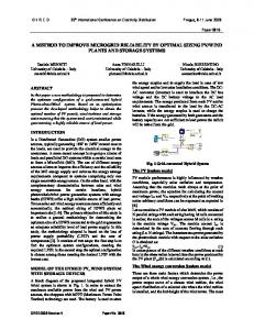
periodically updates TA values. The TA value is often employed by geo-location algorithms in TDMA cellular networks since it is readily available, and gives a good indication of the distance of the mobile from a serving base station. TA values in GSM, however, are fairly coarse, having a theoretical resolution of 554m. Consequently, many points in the cell area will have a common TA value. In practice, the resolution of the TA may be further degraded by multi-path and fading. Figure 1 illustrates the Cell ID-based method where the small gray circles denote the estimated mobile position. We define the following notation: cell radius (R), distance between the mobile and the base station (r), distance between the actual mobile position and the estimated mobile position (d), distance from the base station to the estimated mobile position (r0), and the angle formed by r, r0 and d (θ).

where

d 2 = 2r 2 (1 − cos θ ). Basic TA yields an RMS error of 800m (2000m) for a cell with a 5km radius and an overlap angle of 30° (0°). We note that the one-way delay value is characterized by the Timing Advance (TA) in GSM, the Round Trip Delay (RTD) in CDMA, and the Round Trip Time (RTT) in UMTS. Thanks to this analogy, the circular belt defined by the TA value can be extended to RTD in CDMA and RTT in UMTS within ±σ, the standard deviation due to randomized measurement errors, and all analytical results apply.

θ=π/6

Reported θ=0 Position

MS Position rdrdθ θ

π/3 R R

r

d

θ=0

d

γ

θr o centroid

d centroid

R

(a)

θ=−π/6

α

rθ BTS

−π/3-

∆TA = 554m

R

(b)

Figure 1: The Cell ID method applied to: (a) an omnidirectional cell, and (b) a three-sectored cell

β

Assuming that the mobile is equally likely to be at any of the locations within the cell, the average Root-Mean-Square (RMS) error for 1(a) is 0.707R and for 1(b) is 0.443R. If the TA value is available as well as information on the set of pilots visible to a mobile, an algorithm we call “Basic TA” can offer enhanced performance over the Cell ID method. Basic TA takes advantage of deployment scenarios in which coverage areas of sectors overlap (as is often the case to improve the likelihood that handovers are successful). In Basic TA, an assessment is made based on mobile-reported pilot measurements, whether a mobile is in a sector overlap region, or a region where neighboring sectors should not be visible by the mobile. The Basic TA algorithm then returns the centroid of the appropriate region, as illustrated in Figure 2. With an overlap angle of 30°, the RMS error of the Basic TA estimate is: π

∫ ∫ 6

RMS error =

−π 6

R

0

2r 2 (1 − cosθ ) ⋅ rdrdθ π

∫ ∫ 6

−π 6

R

rdrdθ

0

0-7803-7467-3/02/$17.00 ©2002 IEEE.

= 0.160 R.

Figure 2: Basic TA method for a cell with 30°° of sector overlap. Estimated mobile position is based on the TA values as well as the set of visible pilots reported by the mobile III. BAYESIAN ESTIMATION This paper presents a solution to yield improved geolocation accuracy compared to the methods described in section II. In this solution, a cell area is partitioned into a grid, and signal strength measurements from neighboring base stations are used to infer which grid point is the most likely position of the user. Our approach is motivated by earlier work done for CDMA systems [8]. The TA value is initially used to determine a set of feasible locations for the mobile. We then assign a uniform prior to this set of locations, and utilize a sequential Bayesian procedure to derive a sequence of predicted locations based on the signal strengths reported by the mobile. After each measurement report, a posterior distribution is available which provides a probability that the mobile is at each of the feasible locations,

1022

given the set of measurements reported by the mobile up to that moment. The most likely location of the mobile is the mode of the posterior distribution. Our method, while similar to database matching methods, differs in a significant way. We use the analytical model in [9] that incorporates distance loss and shadow fading to model the RF environment. The three parameter model only needs to be tuned to particular RF environments by use of a small number of sample RF measurements. (We will show later that the performance of the algorithm is relatively insensitive to the assumed model values.) In contrast, database lookup approaches require extensive measurements of the entire targeted RF environment, at the benefit of improved accuracy. (We note, for example, that the model does not capture canyon effects and other real-world RF phenomena that would be captured through drive test measurements.)

Rk ( x, y ) =

Pk Ak ( x, y )

2

β [ d k ( x, y )]

α

× e −σ s / 2 e − χ k ( x , y )

where the first factor represents the expected signal attenuation due to the path loss and the second factor represents shadow fading. Here, Pk denotes the total power being transmitted on BCCH k, Ak ( x, y ) and d k ( x, y ) respectively denote the antenna gain for BCCH k and the distance between the base station associated with BCCH k and the location ( x, y ) . The constants α and β define the precise nature of the power law for distance loss, and the quantity χ k ( x, y ) denotes a Gaussian random variable with mean zero and variance σ s2 . Fast fading was not incorporated in the model since such effects are averaged out in the measurements reported by mobiles. Let R = (R1 , R 2 , L , R K ) where Ri is given by

Actual mobile location

 RSLi if RSLi > Roi Ri =   0 if RSLi < Roi

TA belt

with RSLi denoting the received signal strength on BCCH i, and Roi is the receiver sensitivity threshold. Suppose P0 ( x, y ) , the prior probability that the mobile is at ( x, y ) is equal to 1/ N where N represents the number of grid points in the domain defined by TA the belt. Then, the probability we find the mobile station (MS) at position ( x, y ) given one set of BCCH measurements is

P1(x, y) = Pr MS at (x, y) | R1  ~ Pr  R1 | MS at (x, y) P0 ( x, y)

Figure 3: Search area of the Bayesian method The implementation cost of the proposed algorithm is kept low by utilizing a mathematical model for the conditional distribution (given a gridpoint) of the signal strength measurements. A sequential Bayesian updating scheme is used to identify the grid point within the TA belt (see Figure 3) that is the most likely position of the user. Three parameters are required for the proposed scheme. Two of the parameters correspond to the path loss component and one corresponds to the shadow fading component of the conditional signal strength distributions, respectively. The input data to the scheme when applied to GSM is the set of BCCH (Broadcast Control CHannels) signal strength measurements of the serving and neighbor cells that are regularly provided by the mobile.

Assuming the pilots are independent of one another, the first update step gives a posterior distribution of k

P1(x, y) ~ PrR1 | (x, y) = ∏ Pr [ Ri | (x, y) ] i =1

Considering pilot visibility, Pr [Ri | ( x, y )] can be written as δi 1−δ i Pr [ Ri | ( x, y ) ] = f RSL ( RSLi ) FRSL ( Roi ) , where i i

1 if RSLi > Roi 0 otherwise

δi =  is

An analytical model for signal strength measurements is described in [9]. Here, we utilize that model but assume that the fast fading factor has been removed through averaging. The resulting signal strength received at grid point ( x, y ) from BCCH k is then

0-7803-7467-3/02/$17.00 ©2002 IEEE.

an

indicator

variable

for

pilot

visibility.

−σ s2 / 2 χ i ( x , y )

Writing RSLi = Ci ( x, y )e e , where Ci ( x, y ) is used to represent the distance loss component, we obtain

1023

f RSLi ( RSLi ) =

1

σ s 2π

2

e

− σ s2 / 2 + log RSLi − log Ci ( x , y )  / 2σ s2  

1 RSLi

Error sample points for the Bayesian method were generated by randomly placing a mobile in the serving sector. RF signal strength measurements of the serving and interfering sectors were constructed by attenuating the signal with the distance dependent path loss component and i.i.d. log-normal shadow fading components. The error of each position method was calculated. A path loss exponent of 3.6 was assumed for all results presented.

σ / 2 + log Roi − log Ci (x, y)  FRSLi (Roi ) = Φ   σs   2 s

2

e −u du . It follows that the posterior

2π −∞ distribution for the location of the mobile is proportional to

Figure 4 shows cumulative distribution functions of the geolocation error for the Bayesian update method under different degrees of log-normal shadowing for a cell with radius 5km. We note that even under the moderate log-normal fading conditions typical relatively open spaces like rural and sub-urban environments (2dB), the method cannot satisfy the stringent requirements of the FCC mandate.

δi

2  − σ s2 / 2 + log RSLi − log Ci ( x , y )  / 2σ s2   1  P1 ( x, y ) ~ ∏  e   i =1  σ   s 2π

1− δ i

.

Normalizing so that ∑ P1 ( x, y ) = 1 gives the exact posterior

1

( x, y )

2

M ( x, y ) = − ∑ δ i σ s2 / 2 + log RSLi − log Ci ( x, y )  / 2σ s2

σs=2 dB

σs=4 dB

0.7

σs=0 dB

0.6

σs=6 dB

0.5 0.4 0.3

TA granularity: 554.0 m Cell radius: 5.0 km Grid: 100 m

0.2

i =1

0.1

 σ 2 / 2 + log Roi − log Ci ( x, y )  + ∑ (1 −δ i ) log Φ  s  i =1 σs   K

5400

4800

4200

3600

3000

2400

1800

600

1200

10

0 250

K

0.8 Pr[position error