A biologically inspired model adding binaural aspects to soundscape analysis Michiel Boes1, Bert De Coensel2, Damiano Oldoni3, and Dick Botteldooren4 Acoustics group, Department of Information Technology (INTEC), Ghent University Sint-Pietersnieuwstraat 41, 9000 Gent, Belgium
ABSTRACT Binaural hearing is an essential property of the human auditory system. It is providing the brain with vital information about the location of sounds and this information contributes to the process of auditory stream segregation. Thus, models for the computational analysis of soundscapes would benefit from the addition of a binaural component. In this paper, a biologically inspired binaural analysis model is presented. The neural pathways in the human brain calculating interaural time difference (ITD) and interaural intensity difference (IID), two essential binaural cues, are modelled. Consequently, a neural map is used to link these ITD-sensitive and IID-sensitive neurons to neurons representing a specific direction, in order to obtain an estimate of sound source direction. This map turns out to be both a biologically plausible and an elegant way to combine IID and ITD information. The model is shown to incorporate learning and adaptation in localization as well as several other features of human binaural hearing. In addition, an analysis is presented of the model's effectiveness in detecting sound source directions, also in the presence of distracting sounds or background noise. Keywords: binaural hearing, sound localization
1. INTRODUCTION To structure the auditory environment, the human auditory system tries to determine what produced a perceived sound and where this sound source is localized. These are essential skills i n human auditory scene analysis [1-2]. In particular, sound localization information is considered to be very important for the human brain in order to separate sound sources in a multiple -source acoustic environment (the so-called Cocktail Party Problem) [3]. Thus, also for computational auditory scene analysis, a sound localization component can provide important information. In this paper, a biologically inspired binaural analysis model is presented. In section 2, a short overview of current knowledge on sound source localization in the human brain is given. The proposed model for computational sound source localization, inspired on the human system, is then presented in section 3. In section 4, the model is applied to a selection of test cases. In section 5, our conclusions are presented.
2. HUMAN SOUND SOURCE LOCALIZATION For sound source localization in the horizontal plane, the human brain makes use of two important cues: Interaural Time Difference (ITD) and Interaural Intensity Difference (IID). ITD is caused by the additional time needed for the sound wave to reach the ear furthest to the sound source, whil e IID is caused by the shading effect of the head [1-4]. While these cues are very important in horizontal localization, they are virtually useless in vertical localization. In order to achieve vertical localization, the brain makes use of monaural, spectral cues, caused by the dependence on the sound’s direction of 1 2
3 4
[email protected] [email protected] [email protected] [email protected]
1
incidence of diffractions and reflections on the external ears, head and shoulders [1-5]. In what follows, we give a simplified overview of how these cues are calculated and represented in the human auditory system. Incoming sounds are transferred via the outer- and middle ear to the inner ear, where they are splitted up into different frequency channels by the cochlea. From this point, the system is tonotopically organized, meaning that the different frequency channels are further processed by separate neural circuits, parallel to each other, sensitive to only a limited frequency range around their characteristic frequency (CF). Hair cells convert the pressure signals in the cochlea into electrical signals to be transferred to the brain via the auditory nerve. The brain zone that is thought to be encoding ITD is the medial superior olive (MSO). It receives excitatory input from both ears. Several models for explaining ITD sensitivity of MSO cells exist, the classical being Jeffress’ delay line theory [6]. In this model, the MSO performs a calculation somewhat similar to a cross-correlation between the inputs from the two ears. IID is encoded in the lateral superior olive (LSO). This brain zone receives excitatory input from one ear, and inhibitory input from the other ear, and its output is related to the difference in intensities of the two ears [1].Monaural cues are thought to be encoded in the dorsal cochlear nucleus (DCN) [5]. Cells encoding these localization cues mainly project to the Inferior Colliculus (IC) and further via the medial geniculate body (MGB) to the auditory cortex [7]. It is not yet completely clear what exactly happens in these zones, but a conversion from the localization cues to a location estimate is necessary.
3. MODEL 3.1 Preprocessing First, time intervals of a fixed duration are extracted from the incoming sound sample. These intervals may overlap. The obtained fragments are then sent through a filterbank, imitating the frequency decomposition effect of the cochlea. Using this windowing in both the time domain and the frequency domain, we split the incoming signal up into an array of sound samples with limited time and frequency range. These sound samples are then analyzed and localized individually. In order to simulate the effect of the hair cells, the signals are half-wave rectified, and the resulting signal is converted to a logarithmic scale to take into account the effect of the auditory nerve. 3.2 Localization features Next, the response of MSO and LSO neurons to the incoming sound samples is simulated. A first approximation is the use of cross-correlation to simulate the sensitivity of MSO neurons to ITDs. The output of a neuron with maximal response at an ITD of T will then be represented by the value of the cross-correlation function of the input from both ears at a time difference of T. Thus, by calculating the cross-correlation function of the input signals at both ears, we have simulated the output of an array of MSO neurons with maximal response at different ITDs. The response of LSO neurons can, in a first approximation, be modeled as arctan(Isignal - I neuron), with Ineuron the characteristic intensity difference of the simulated neuron, and Isignal the calculated intensity difference (in dB) of the incoming sound. It has been suggested that MSO neurons are actually sensitive to interaural phase difference instead of interaural time difference [8]. The model of MSO neurons described above can easily be adapted in order to implement this. Because the sound samples that are analyzed only have a limited frequency range, it is reasonable to convert time difference to phase difference using the central frequency of each frequency band. Monaural cues are not taken into account in this paper, as we are mainly concerned with sound localization in the horizontal plane. 3.3 Mapping Subsequently, the outputs of all simulated MSO and LSO neurons are grouped into one localization feature vector. With this vector, a sound source direction can be estimated, using a mapping between localization feature vector-space and location-space. To implement this mapping, a simple Bayesian system is used. We define theta as the angle in the horizontal plane where the sound originates, T i with i an integer between 1 and M are intervals into which the angle space ]0°,360°] is divided, fq are localization feature vector element values and Fq,jq are intervals in which the localization feature vector element value space is divided. Using Bayes'
2
theorem, it is then found that:
P( Ti | f1 F1, j1 ... f N FN, jN ) = =
P(f1 F1, j1 ... f N FN, jN | Ti )P( Ti ) P(f1 F1, j1 ... f N FN, jN ) P(f1 F1, j1 ... f N FN, jN | Ti )P( Ti ) M
P(f k 1
1
(1)
F1, j1 ... f N FN, jN | Tk )P( Tk )
In a next step, the assumption that all localization feature vector values are statistically independent is introduced. Although these values clearly are not statistically independent, this approximation will prove to be producing satisfactory results. We get:
P( Ti | f1 F1, j1 ... f N FN, jN ) =
P(f1 F1, j1 | Ti )... P(f N FN, jN | Ti )P( Ti ) M
P(f k 1
1
(2)
F1, j1 | Tk ) ... P(f N FN, jN | Tk )P( Tk )
We can evaluate this expression if we have values for P(θT i) and P(f qFq,jq | θ T i) for all q, j and i. P(θ T i) can be considered equal for all i (and thus equal to 1/M), or can be determined by a priori knowledge about possible locations of the sound source. P(f qFq,jq | θ T i) can be estimated by training with recorded sounds originating from directions with θ T i. As a training set, an array of real broadband sounds (airplanes, crying babies, ...) is used. These are recorded by an artificial head, with the sound source placed at a certain θ, and at a distance of about 3m. This was repeated 36 times, sampling the horizontal plane at all integer multiples of 10°. Subsequently, these sounds are analyzed as described in sections 3.1 and 3.2, and for every recorded value of θ, an array of localization feature vectors is obtained. Using these vectors, a Gaussian probability distribution for each vector element can be estimated and this can be used to evaluate P(f qFq,jq | θ T i). In the calculation of the parameters of the Gaussian distribution, features associated with more intense input in the corresponding frequency band are given more importance, as features associated with less intense input in that frequency band may be dominated by noise.
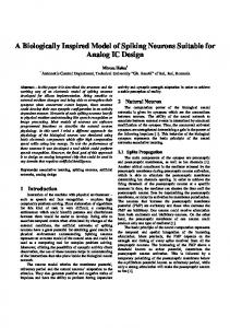
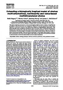
4. RESULTS An interesting way of visualizing the results of the localization model described in section 3 is to display detected sound source direction as a function of time and frequency. Thus, for each time-frequency window as described in section 3.1, a sound source location estimate is calculated as an average of sound source directions, weighted by their calculated probabilities. In figure 1a, a spectrogram of a recording of a police siren is shown. In the recording, the sound source is located at an angle of 50° (with -90° defined to be to the left, 0° right in front and 90° to the right of the artificial head). Figure 1b shows the first results of the location analysis. This does not look very good, because the system has difficulties distinguishing between front and back. Humans mainly use monaural cues to sense the difference between front (θ) and back (180°- θ), as ITD and IID are nearly the same for these angles [5]. Thus, because we omitted these monaural cues in our model, it is very natural that this problem occurs. When the color scale of the plot is changed in such a way that angles θ and 180°- θ are represented by the same color, in order to eliminate this problem, the result of figure 1c is obtained. The source is now well localized, as a large zone with the color representing 50° (or 130°) can be seen.
3
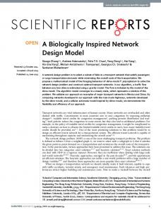
Figure 1 – a: Spectrogram of police siren, positioned at 50°, frequency channels are in 1/3 octave bands, 1 time window every 0.1s. b: Localization of police siren. c: Localization of police siren, without front-back confusion. d: Similar to 1b, but without training at odd multiples of 10°. e: Similar to 1c, but without training at odd multiples of 10°. To simplify comparison, a contour, defining the most intense zone in the spectrogram, has been added on all figures. In the previous example, the test sound originated from an exact direction at which the system had been trained (as it was trained at all multiples of 10°). In order to test whether the system still works with incoming sounds originating from directions in between trained directions, now an analysis is presented of the same sound as before, but taking into account only training data of all multiples of 20°. Similar plots as in the previous example can be found in figures 1d and 1e. It can be seen that localization is still good, but with more front-back confusion. In the next cases, front-back confusion will be eliminated, like in figures 1c and 1e. As a second example, a recording of an airplane at a fixed angle of 50° is considered. The spectrogram of this recording can be seen in figure 2a, and the result of the location analysis in figure 2b. It can be seen in the figure that localization at low frequencies, below channel 5, or below about 200Hz, is not good. This is caused by the fact that, at these frequencies, wavelengths are longer than 1m, while the distance between the two ears is only about 20cm. Because of this, ITD’s become increasingly difficult to perceive as the frequency decreases. In addition, at these low frequencies,
4
there is almost no shading effect of the head, so IID cues also become useless. The use of different features might possibly ameliorate localization at these low frequencies, but, when tested with interaural phase difference instead of interaural time difference in the localization feature vector (as explained in section 3.2), no improvement is observed.
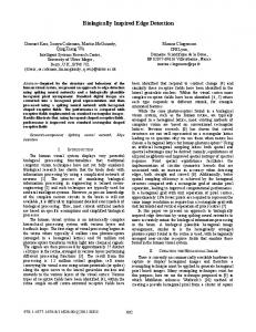
Figure 2 – a: Spectrogram of airplane sound, positioned at 50°, time and frequency scales as in figure 1. b: Localization of airplane sound. c: Localization of airplane sound, only using ITD cues. d: Localization of airplane sound, only using IID cues. As in figure 1, a contour has been added for easy comparison of the figures. In figure 2c, the result of localization analysis in which only MSO neurons, representing ITD information, were taken into account, is shown. Overall, results are still quite good, but mainly at higher frequencies the localization quality deteriorates. In figure 2d, the result in which only LSO neurons, encoding IID information, are used, can be seen. Localization in this case is a lot worse. These figures show that in the model, ITD information dominates localization, and IID information becomes important at higher frequencies. This corresponds to observations in human sound localization, and agrees with the classic duplex theory of Thompson and Rayleigh, which states that ITD is used mainly at lower frequencies while IID is used mainly at higher frequencies [1-4]. Finally, it is shown how this localization model can be applied to improve sound source detection and auditory stream segregation. For this purpose, the police siren analyzed in figure 1 is superimposed on white noise. Figure 3a shows the signal to noise ratio in dB (SNR dB) for each time-frequency window and figure 3b shows the results of the localization analysis on this signal. It can be seen that time-frequency windows with a high SNR dB are localized correctly, while windows with a low but positive SNR dB are not localized perfectly but still stand out of the white noise background, which is located more or less around 0°. It is clear that th is localization information can be of used to select time-frequency windows with positive SNR dB, and thus help sound source detection in a noisy background.
5
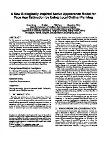
Figure 3 – a: Signal to noise ratio in dB of a police siren (located at 50°) in white noise, time and frequency scales as in figure 1. b: Localization of the police siren in white noise. For easy comparison, a contour at a SNR of 5dB is added. Now, the sound of the police siren at -20° is superimposed on the sound of footsteps at 70°. The ratio of the first signal to the second signal for each time-frequency window is shown in figure 4a. Figure 4b shows the resulting angles. It is clear that in windows where one of the two sources is dominating, this source is well localized. By grouping time-frequency windows originating from the same direction, basic auditory stream segregation can be accomplished, or this localization information can be used to help in the process of stream segregation.
Figure 4 – a: Ratio of police siren (located at -20°) to footsteps (located at 70°) in dB, time and frequency scales as in figure 1. b: Localization of the sound in 4a. For easy comparison, a contour at a ratio of 5dB is added (red) and one at a ratio of -5dB (blue).
5. CONCLUSIONS This paper presents a biologically inspired model for binaural hearing, which is useful for localizing sounds in the horizontal plane. The model displays several features also seen in human binaural hearing, indicating that it is a biologically plausible model. The model also produces useful information for the process of auditory stream segregation, as binaural hearing does for humans. The model can be extended and possibly improved by including monaural features. This could solve the difficulties the model currently has with front-back confusion and even enable it to localize sounds in the complete space, and not just in the horizontal plane.
REFERENCES [1] Tom C.T. Yin, “Neural Mechanisms of Encoding Binaural Localization Cues in the Auditory Brainstem” Chap. 4 in Integrative Functions in the Mammalian Auditory Pathway, edited by R.R. Fay and A.N. Popper (Springer-Verlag, New York, 2002). [2] Simon Haykin and Zhe Chen, “The Cocktail Party Problem,” Neural Computation, 17, 1875-1902
6
(2005). [3] Masanao Ebata, “Spatial unmasking and attention related to the cocktail party problem,” Acoust. Sci. & Tech., 24, 5 (2003). [4] Tom C.T. Yin and Shigeyuki Kuwada, “Binaural localization cues,” Chap. 12 in The Oxford Handbook of Auditory Science – The Auditory Brain (Volume 2), edited by Adrian Rees and Alan R. Palmer (Oxford University Press, Oxford, 2010). [5] Bradford J. May, “Sound location: monaural cues and spectral cues for elevation,” Chap. 13 in The Oxford Handbook of Auditory Science – The Auditory Brain (Volume 2), edited by Adrian Rees and Alan R. Palmer (Oxford University Press, Oxford, 2010). [6] Lloyd A. Jeffress, “A place theory of sound localization,” J. Comp. Physiol. Psychol., 41 (1948) [7] Manuel S. Malmierca and Troy A. Hackett, “Structural organization of the ascending auditory pathway,” Chap. 2 in The Oxford Handbook of Auditory Science – The Auditory Brain (Volume 2), edited by Adrian Rees and Alan R. Palmer (Oxford University Press, Oxford, 2010). [8] David McAlpine and Benedikt Grothe, “Sound localization and delay lines – do mammals fit the model?,” Trends in Neurosciences, 26, 7 (2003).
7