Obstacle Avoidance. 1. R. Glasius. A. Komoda. S. Gielen. Department of Medical Physics and Biophysics,. University of Nijmegen, Geert Grooteplein Noord 21,.
A Biologically Inspired Neural Net for Trajectory Formation and Obstacle Avoidance. 1
R. Glasius
A. Komoda
S. Gielen
Department of Medical Physics and Biophysics, University of Nijmegen, Geert Grooteplein Noord 21, 6525 EZ Nijmegen, The Netherlands,
Abstract
A biologically inspired two-layered neural network for trajectory formation and obstacle avoidance is presented. The two topographically ordered neural maps consist of analog neurons having continuous dynamics. The rst layer, the sensory map, receives sensory information and builds up an activity pattern which contains the optimal solutions (i.e. shortest path without collisions) for any given set of current position, target positions and obstacle positions. Targets and obstacles are allowed to move, in which case the activity pattern in the sensory map will change accordingly. The time-evolution of the neural activity in the second layer, the motor map, results in a moving cluster of activity, which can be interpreted as a population vector. Through the feedforward connections between the two layers, input of the sensory map directs the movement of the cluster along the optimal path from the current position of the cluster to the target position. The smooth trajectory is the result of the intrinsic dynamics of the network only. No supervisor is required. The output of the motor map can be used for direct control of the actuators of a biological limb or robot manipulator. Even if an external force acts on the limb or manipulator the system is able to reach one of the targets. Computer simulations of a point robot and a multi-joint manipulator illustrate the theory.
1
This work has been submitted to 'Biological Cybernetics' (june 1994).
1 Introduction One of the main themes of research on robot control deals with the issue of trajectory planning and formation. The aim of this research is to develop algorithms which allow multi-joint manipulators to move in a cluttered environment, which may change as a function of time, to multiple targets along a path without collision. The rst steps to deal with this problem were based on global methods which can be considered as a search process for a path in a graph which represents the accessible paths along objects [2]. This approach is practically useful only in a static environment, since the time to construct a graph and to perform the planning task becomes excessively long for a large number of obstacles. As an alternative the idea of potential elds was proposed in which the target acts as an attractor in the midst of obstacles represented by repelling potentials [18, 20]. Unfortunately, the potential eld methods su�ered from several problems, one being that of undesired local minima. Although several suggestions have been presented to circumvent these problems [1, 3, 6, 27, 32], no algorithm was presented which guarantees an exact solution. Glasius et al. [12] proposed a neural network with continuous dynamics that also su�ers from local minima. However, it improves upon previous models in the quality of the path which is smooth and continuous and which is the simple result of the intrinsic dynamics of the network only. In another approach a neural-network type was proposed [7, 24, 30] in which neurons with lateral interactions are positioned on the nodes of a grid. Due to lateral interactions activity from the target spreads through the network (except towards neurons representing obstacles). The optimal trajectory to the target is found by the sequence of neurons which is obtained by stepping along the steepest gradient to the peak of activity in the network, i.e. the target. Although this procedure is shown to give the optimal path, it is not an unsupervised method, since it requires an external observer to compare the activities of neighboring neurons in order to decide which neuron should be the next in the path towards the target. Recently, variations of this distance-transform or wave-propagation method has been proposed [11, 28]. Although supervised methods can be useful for applications, they cannot be used for biologically plausible models for trajectory planning and formation. However, topographically ordered neural networks are frequently found in the nervous system and as such the models by Glasius et al. [11, 12] and Prassler [28] have a biologically plausible basis. In this paper we present a modi cation which has the property that it guarantees a trajectory from any initial position to a target (if one exists) given any arbitrary environment with obstacles, which are allowed to change position. This trajectory is the shortest path in terms of the metric of the representation. This is achieved by proposing two layers with neurons, each with more or less the same properties. This paper is organized in the following way. First we will describe the model and we will prove that the model will nd the shortest path in an unsupervised way. The theoretical results will be supported by numerical computer simulations, which will show the performance of the model for non-trivial problems of trajectory planning. In the discussion we will compare the results of the model with those of previous models. We will also discuss to what extent the model can be used as a biologically plausible model which captures the results on trajectory planning in the neuro-physiological literature and which can be used to propose some new hypotheses. 1
2 The Model The model which we will present, can be used for path planning and trajectory formation in a nite (D-) dimensional con guration space of any system. This could be a multijoint limb, in which case the joint-angles of the limb can be represented as a vector in the D-dimensional con guration space C , or a multi-joint robot manipulator. Let us regard a topographically ordered neural map in which the activity of each neuron i is related to a subset in C , called the receptive eld rfi of neuron i. Related to the topographical ordering, neighboring neurons have neighboring receptive elds in C . Each receptive eld rfi can be represented by a D dimensional vector �i, which points to the center of the receptive eld. Hence, to each neuron i corresponds a receptive eld rfi and a vector �i. If the receptive elds cover the complete con guration space,
C=
N [
i=1
rfi
(1)
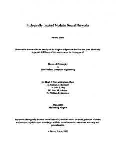
then the grid consisting of all �i is a discrete representation of the con guration space C . Topographically ordered neural maps can be obtained in several ways (for example by Kohonen's topographically ordered maps [19, 29] or by a vector-quantization learning rule [9, 25, 29]). Such topographically ordered maps are used in both layers of our neural network model. The rst will be denoted as the "sensory map", because it is assumed to represent information about the environment of the system. The other map will be referred to as the "motor map", because its activity codes action commands. To distinguish the variables and parameters between the two maps, the variables and parameters in the sensory map will have indices i and j and those in the motor map k and l. The sensory map projects to the motor map with feedforward connections which will be de ned later (see Eq. 8). For a two-dimensional system the architecture of the neural network containing the topographical maps and the connections are illustrated schematically in gure 1. The activities of the neurons in both maps are characterized by real-valued variables �i; �k 2 [0; 1] where �i denotes the activity of neuron i in the sensory map and �k that of neuron k in the motor map. The input to a neuron, the local eld, is de ned as the weighted sum of the activities of all other neurons in the network minus a threshold. The local eld for neurons is denoted in the sensory map by ui and for neurons in the motor map by uk . The neuron activity is given by the value of a sigmoid function on the local eld. Our choice for the sigmoid function is 8 > < 0 if x � 0 (2) g (x) = > x if x 2 [0; 1] : 1 if x � 1 with > 0. However, it could be any bounded function between 0 and 1 which is monotonically increasing. Consequently, the neuronal activities are �i (t) = g (ui (t)) for neurons in the sensory map �k (t) = g (uk (t)) for neurons in the motor map 2
Current Position
Target Position
Sensory map
cle
sta
Ob
Feedforward Projections Motor map
Command Position
th
Pa
Figure 1: A schematic representation of the two-dimensional sensory map and motor map as a two-layer feedforward neural network.
3
2.1 The Sensory map
We assume lateral excitatory short-range connections Bij from neuron j to neuron i in the sensory map: Bij = f (j�i ? �j j) (3) where f (x) is a monotonically decreasing neighborhood function and j�i ? �j j is the Euclidean distance in con guration space between �i and �j . By example a commonly used [21, 22, 23] function is ( ? x2 if jxj 2 [0; r] e f (x) = 0 (4) if jxj > r with and r real positive numbers. External input is assumed to provide information about target and obstacle positions. The state of the neuron which represents the target con guration in C , is supposed to be close to or equal to the value "1", i.e.maximally activated. We will call this neuron the target neuron. Similarly, due to inhibitory connections from external sensory inputs, the set of neurons which corresponds to the positions of the corresponding (forbidden) con gurations, are supposed to be de-activated, i.e. in state "0". Because target and obstacles may move as a function of time, the neurons representing the target and the set of obstacle neurons may be changing continuously. In conclusion, the external sensory input to neuron i in the sensory map is given by 8 > v if target 2 rfi < Ii = > ? v if obstacle 2 rfi (5) : 0 otherwise where v is a positive number, large enough to dominate over all other inputs. The threshold of the neurons in the sensory map is set to zero. The total input to a neuron in the sensory map is given by
ui (t) =
N X j
Bij sj (t) + Ii
The dynamics for the neurons in the sensory map can be formulated by the change of the neural inputs ui per unit of time N dui (t) = X Bij sj (t) + Ii ? ui (t) (6) dt j The function
X X X L (�i) = ? 21 Bij �i sj ? Ii�i + G (�i )
i;j
R �i ?1 g (x) dx,
i
i
with G (�i ) = is a global Liapunov function [11, 13, 15] for the sensory map. The existence of a Liapunov function guarantees that the dynamics of the sensory layer always converges to a xed point. Due to the excitatory local interactions, the target neuron, kept at a high activity, feeds its nearest neighbors through the short range connections, such that the activity 0
4
spreads through the network. As shown before [11] the activation landscape which arises in the sensory neural map, is shaped like a hill with its top at the target neuron and with valleys at the locations of the obstacle neurons. Therefore, for each given initial position, target position and the set of obstacles, the optimal solution is the path constructed by successive gradient ascents to the top and the sensory map contains all solutions given the set of obstacle and target neurons. This neural activity eld is passed to the motor map neurons, and, in addition, neurons in the motor map receive an external input which codes the current con guration of the system. The motor map has to construct a motor command which will alter the current con guration in a direction along the path towards the target. In the case of moving objects, the set of obstacle neurons and the set of target neurons may change continuously in time. The activation landscape in the sensory map changes accordingly and if the obstacles move slowly relative to the time constant of the system dynamics, then the sensory map will always contain adequate information to the path planning problem.
2.2 The Motor map
The motor map receives inputs through feedforward connections from the sensory map. In addition, the motor map receives input which provides information about the current actuator con guration. This input could originate from sensors in the actuators of the limb or manipulator. With both input signals the motor map is able to produce motor commands which will continuously change the current con guration of the actuator such that it moves from the initial position to the target position. The motor map has both short range and long range lateral interactions. The short range excitatory interactions are the same as those in the sensory system: Bkl = f (j�k ? �l j) The lateral long-range interactions are inhibitory with strength ( J 0 if i 6= j , with J 2 IR Jij = 0N otherwise A motor P neuron k has a constant threshold of J � ? l2Bkl ? � (7) where � 2 IR and � 2 IR are constants. From formula (7) it follows that each neuron k can have a di�erent threshold. In biological perspective, we could make the interpretation that a "large" neuron, i.e. having a large number of connections, has a large threshold. However, if the neurons are homogeneously distributed over the con guration space then all neurons have the same number of neighbors. This results in all neurons in the motor map having the same threshold. Each con guration � 2 C of the actuator is represented in the sensory map and in the motor map. The connections from the sensory neuron i to the motor neuron k are given by (8) B^ki = P �B f^ (j�k ? �i j) j kj 0
+
0
+
5
where f^ (x) is similar to f (x) and � is the same constant as in (7). These connections provide part of the input signals to the motor map. The other part has an external origin. It supplies an input with magnitude Kk (�A) � ?v + v f~ (j�A ? �k j) (9) where �A represents the "current manipulator position" in con guration space and where f~ (x) is a similar function as f (x) with ~ < and with r~ > r. The large inhibitory input ?v suppresses all other inputs to neurons in the motor map with a receptive eld at a distance larger than r~ from the current manipulator position. Therefore the activity of these neurons is close to the minimal output value of the sigmoid function g. With this particular combination of inputs to the motor map and within a certain range of parameters, it is our intention to localize the activities in the motor map into a cluster with an almost constant size. The cluster of activities has to move over the map in a direction supplied by the inputs from the sensory map. In that case we can interpret the symbolic content of the clustered activities in the motor map by means of the following de nitions of some macroscopic variables. We de ne the "mean total activity" m X m � N1 �k (10) k Then we de ne �B as the "command manipulator con guration" P k �k �k (t) �k (t) �B (t) � P (11) k �k (t) �k (t) with �k (t) � [1 + sgn (�k (t) ? � )]. This is the weighted mean of all centers of receptive elds of motor neurons that have an activity larger than a certain activity threshold � . A neuron belongs to this set if �k is nonzero. The vector value �B (t) is the output of the system which is sent to the actuators as a command to realize this con guration. However, it takes some time before the actuators receive and realize the command con guration. Therefore, the command manipulator con guration points to the con guration what will be the current con guration after that period of time. The command position always leads the current position until it nally reaches the target con guration. Because the target con guration �T (t) may move in time, more information can be provided using relative coordinates with respective to the target con guration instead of absolute coordinates. Therefore we de ne the "relative command manipulator con guration" X
X � �B ? �T
Similarly, this vector can be de ned as a weighted mean: P X (t) � k Pxk (�tk) (�t)k (�tk) (�t)k (t) (12) k with xk (t) = �k ? �T (t) as the position in con guration space of motor neuron k relative to the target position. The relative command manipulator con guration X is the weighted mean of all relative vectors of motor neurons that have an activity larger than a certain 6
activity threshold � . In this perspective we can regard this variable X as a population vector. The output of the motor map can be regarded as a motor command. In the case of a spring-like muscle system, each manipulator con guration can be accomplished by de ning a particular set of spring constants [4, 14] or rest lengths [8] of the spring-like muscles. If each motor neuron k sends a motor command proportional to �P t �� tt �� tt , then the command manipulator con guration is a motor command consisting of votes of individual neurons to move the actuator to a certain con guration �B . When the cluster moves smoothly, a continuous stream of motor commands is generated by the motor map which can be used for direct control of the actuators. k(
k
)
k(
k(
) k( )
) k( )
The total input to a motor map neuron is given by ! P P X B � ki i i uk (t) = Bkl�l ? J (m ? �) ? � 1 ? P B + Kk (�A) ? l2Bkl i ki l 0
As explained before [12] each term in this expression has a di�erent e�ect on the behavior of the network. The term J (m ? �) tends to set the number of active units such that P m = �. The local neighbor interactions l Bkl �l make it more advantageous for neighboring units to be active. Therefore, this term tends to impose clustering of the active units. The clustering prevents that an obstacle neuron is surrounded by active neurons. Rather the cluster avoids the obstacle; it behaves as if the cluster possesses some kind of surface tension. The external input, causes the cluster to move to the maximum of that input which is the target position ( �i � 1 in the sensory map). The external input Kk (�A) makes sure that the cluster, i.e. the command position, is near the current position. 0
If the following substitutions are made (13) Tkl � Bkl ? JN ! P P B � ki i i Ik � J � ? � 1 ? P B + Kk (�A) ? l2Bkl i ki then the equations for the input of the motor neurons are similar to the equation for the input of the sensory neurons. 0
0
uk (t) =
N X l
Tkl �l (t) + Ik
Hence, the dynamics for the neurons in the motor map are similar to the dynamics of the neurons in the sensory map N duk (t) = X Tkl �l (t) + Ik ? uk (t) dt j
(14)
resulting in a similar structure for the Liapunov function, X X X L (�) = ? 21 Tkl �k �l ? Ik �k + G (�k ) k;l k k 7
with G (�k ) =
R �k ?1 g (x) dx 0
.
The system has the ability to react to external forces acting on the manipulator. If an external force suddenly changes the con guration of the manipulator, then the current position jumps to a new location. Consequently the external input Kk (�A) changes and causes an inhibition at all positions excepts in the neighborhood , characterized by r~ of f~ in (9), around the new current position. If the command position XB is outside this region then the cluster disappears due to the inhibition and reappears at the location with the highest local eld. Therefore, a change of the current position is followed by a change in the command position. The new command position gives the manipulator the command signals to move to the new command position, which is close to the new current position. If a continuous force acts on the manipulator, such that the current con guration does not jump but merely shifts in the con guration space, the cluster movement is not only due to the motor system but also due to the external force. The cluster however, is always trapped in the vicinity of the current position, i.e. the area de ned by r~ of f~, and is always on the optimal path to the target con guration. Hence if the force produced by the actuators is strong enough to dominate over the external continuous force then the target will be reached. The length r~ depends on the time delays in the motor system and on the velocity of the manipulator. It takes some time to send the motor command from the motor map to the actuators, to move the actuator and to send the new current position back to the motor map. Consequently the current con guration is always a moment of time �t behind the command con guration. Depending on the velocity of the cluster in the motor map, as a result of the system dynamics, the length r~ in con guration space can be calculated such that the command con guration is never further away than the cluster can move in a time �t. The result of the combined interaction of the terms, is a cluster of activities in the neural motor map, moving continuously and smoothly in the direction of the gradient of the local dragging eld. It produces motor commands that move the manipulator to the command con guration, which is at most a distance r~ away from the current con guration until the target position is nally reached.
3 Computer simulations
3.1 A point robot in a two dimensional work space
In the rst simulation we regard a point robot moving in a square subset of a twodimensional cartesian work space. The initial position of the point robot is in de cavity of a concave obstacle (see gure 2). The target position is placed at the other side of the obstacle. The sensory map and the motor map are both two-dimensional neuronal maps, consisting of a square lattice of 50x50 neurons with receptive elds that are square-shaped. The receptive elds cover the complete work space according to equation (1) and the maps have the same topography as the work space.
8
The short range lateral connections are characterized by the neighborhood function (
? x? 2 if the distance x between two nodes is greater than zero and less or equal to thr e f (x) = 0 if x = 0 and x > 3 Note that x is discrete corresponding to the distances between the nodes on a lattice. The projections from the sensory map to the motor map are similar but additionally sensory neurons project to motor map neurons with the same receptive elds. 8 if x = 0 > < 1 2 ? x ? ^ f (x) = > e if x 2 h0; 3] : 0 if x > 3 In the projections from external origin to the motor map, equation (9), we chose the neighborhood function
f~ (x) =
(
(
1)
(
1)
e? : 0
x
0 01 2
if x 2 [0; 6] if x > 6
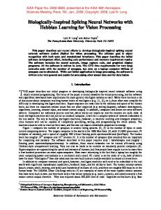
The external inputs to the sensory map are described in equation (5). With v = 1000 in equations (5) and (9) and with = 0:3 in formula (2) of the system dynamics, all parameters for the simulation are set. In the sensory map a peak of activity around the target neuron grows in width. The target neuron, activated by external input to its maximum, activates its neighbors through the short range connections. The neighbors of the target neuron activate their neighbors and so on. In the vicinity of an obstacle neuron, which activity is kept at the minimal value, the spread of activities stops in the direction of the obstacle neuron. The resulting asymptotic neural activity values in the sensory map are shown in gure 3. If target nor obstacle move, then the resulting hill is stable. The neural activity in the motor map at four points in time is shown in gure 4. At all times there is a cluster localized somewhere in the map. Initially the cluster is located at the start position, i.e. in the cavity of a concave obstacle. Then, as a result of the system dynamics only, the cluster moves away from the target, it rounds the obstacle and eventually it moves to the target and reaches it. The path is smooth and continuous.
3.2 Simple connections for real time robot trajectory formation
For robot trajectory formation minimizing the number of connections and simplifying the neighborhood functions enlarges the speed of the software. Moreover, a simpler structure of the network creates the possibility to implement the model in fast analog hardware. Consider a D-link robot manipulator. In this case the con guration space is Ddimensional and can be described by the D joint angles of the links. The structure of both topographical maps is a D-dimensional cubic lattice of neurons. The neurons have a D-dimensional square shaped receptive eld that does not overlap with the receptive eld of other neurons. The receptive elds are contiguous and the map is periodic such that they cover the complete con guration space. Therefore, the centers of the receptive elds are also ordered according to a D-dimensional lattice.
9
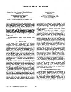
T
I
Figure 2: Representation of work space. Black dots are part of a concave obstacle. The open circle marked with an I is the initial position. The open circle marked with a T is the target position. The neighborhood functions in the lateral short range connections of the two topological maps are ( x 2 h0; r] f (x) = 10 ifotherwise resulting into lateral short range connections that are symmetric with value 1. Every neuron i in the sensory map projects to only one neuron k in the motor neuron which has the same receptive eld. ( x=0 ^ f (x) = 10 ifotherwise The neighborhood function, characterizing the projections from external origin, has been chosen: ( x 2 [0; r~] f~ (x) = 10 ifotherwise The feedforward projections from sensory map to motor map consist of connections with strength � between the corresponding neurons. Let sensory neuron �i k project to motor map neuron �k , then the input partly from the rst layer is ( )
�
?� 1 ? �i k
�
(15)
( )
10
1 0.8 0.6 0.4 0.2 0 50 40
50 30
40 30
20
20
10
10 0
0
Figure 3: Stable neural activity in the sensory map as function of the position of the neurons in the 50x50 neural grid (See section 3.1). The map is isomorphic to the work space in gure 2.
11
1
1
0.8
0.8
0.6
0.6
0.4
0.4
0.2
0.2
0 50
0 50 40
50 40 30
50 30
40 30
20
20
10
10 0
30
20
20
10
40 10 0
0
0
(a)
(b)
1
1
0.8
0.8
0.6
0.6
0.4
0.4
0.2
0.2
0 50
0 50 40
50 40 30
40 30
20
30 20
10
10 0
40 20
20
10
50 30
10 0
0
(c)
0
(d)
Figure 4: Activation landscape in the motor map at four time instances during the movement of the cluster to the target position (See section 3.1). The neuronal map is isomorphic to the work space in gure 2.
12
Conclusively, the input to a sensory neuron is
ui (t) =
N X j
Bij �j (t) + Ii
and to a motor neuron
uk (t) =
X
l
�
�
Bkl�l ? J (m ? �) ? � 1 ? �i k + Kk (�A) ? 0
( )
p
P
l Bkl
2
In the simulation we chose � = 1, D = 2 and r = 2. With a square lattice the last P B term is now = 4. The rest of the parameters as well as the initial position, the target position and the obstacle positions are chosen the same as in the former simulation (see gure 2). The asymptotic stable state of neural activities in the sensory map is shown in gure 5(a). The cluster in the motor map located at the target position is shown in gure 5(b). The di�erences with the results of the rst simulation, due to the simpli ed connections, are the width of the activity hill in the sensory map, which is smaller than that in gure 3, and the cluster in the motor map is more localized as in gure 4(d). The speed of the cluster depends on the slope of the activation hill. Because the slope of the activation hill in the outer region is smaller than in the previous simulation, the speed in system-time-units in this simulation is smaller compared to the previous simulation. However because of the simple connections the time to simulate this system on a sequential computer is far more less than the simulation time for the rst simulation. A more localized cluster has the same total mass of positive activity on a smaller area, which means that the cluster is more dense. The density of the cluster is important when it is in the vicinity of an obstacle. A dense cluster has higher neural activities which makes it more di�cult to enclose obstacles in its area. It results in a larger surface tension such that obstacles can deform the shape of the cluster much harder. Hence the 'point robot' may have some extent, equal to the hard core of the cluster. Nevertheless, the resulting paths in the two simulations are qualitatively equal and we want to stress that the model is quite insensible to the choice of the neighborhood functions. l
kl
2
3.3 Choosing between multiple targets
In the following simulations we regard a two link manipulator working in a two-dimensional work space. To reach any point in work space with the manipulator end-e�ector two con gurations are possible. Hence the system has to chose between two target manipulator con gurations having the same end-e�ector work space coordinates. the rst simulation is without obstacles, the second contains one obstacle in work space. The con guration space of the manipulator can be described by the two joint angles of the manipulator. The neural maps, again, consist of a neural grid of 50 by 50 neurons. Each neuron has a square receptive eld. Because the joint angles are periodic the neuronal maps have to be cyclic. Hence the shape of both maps is that of a torus. The other parameters are chosen the same as in the second simulation described in section 3.2 of the point robot with simple connections. The resulting neural activities on the sensory map are shown in gure 6. Depending on the initial position of the manipulator in con guration space, steepest ascent will lead 13
1 0.8 0.6 0.4 0.2 0 50 40
50 30
40 30
20
20
10
10 0
0
(a)
1 0.8 0.6 0.4 0.2 0 50 40
50 30
40 30
20
20
10
10 0
0
(b)
Figure 5: Stable neural activity as a function of the position of the neurons in the 50x50 neural grid (see section 3.2). Both neural maps are isomorphic to the work space in gure 2. a) The sensory map. Note that the width of the activation hill is smaller than the width of the activation hill in gure 3. b) The motor map. The cluster is at target position. Note that the cluster has the same mass of positive activity on an area larger 14 than that in gure 4(d).
1 0.8 0.6 0.4 0.2 0 50 40
50 30
40 30
20
20
10
10 0
0
Figure 6: Stable neural activity in the sensory map as a function of the position of the neurons in the 50x50 neural grid. a) Two target positions in con guration space correspond to the same manipulator endpoint coordinate in work space. b) An obstacle changes the ow of activities and the resulting landscape. to one of the tops. Both target con gurations have a basin of attraction consisting of all initial positions that will result in a stable end-con guration at that top. In the rst simulation we chose two initial positions one leading to one top and the other to the other top. In gure 7(a) and 7(b) the manipulator has been shown at four di�erent time instances. Note that the end-e�ector target position in both pictures is the same. In gure 7(c) both paths have been shown in con guration space. In this simulation we only add a round obstacle in work space to the former simulation (see section 3.3). All manipulator con gurations which are blocked by the obstacle are called obstacle con gurations. The neurons with an obstacle con guration in its receptive eld are referred to as the obstacle neurons. The obstacle neurons block the activity
ow from both target neurons. The resulting activity landscape in the sensory map is shown in gure 8. Note that the basin of attraction belonging to the target con guration distal to the obstacle is enlarged, while that of the proximal target con guration became smaller (compare gure 9 with gure 7). We choose an initial con guration close to the target con guration proximal to the obstacles. The resulting manipulator movement is illustrated in gure 9(a), the path in con guration space is shown in gure 9(b). Note that in the former simulation this initial con guration would lead to the other target con guration.
15
Ia
Ta
T
T
Tb
Ib
(a)
(b)
(c)
Figure 7: Manipulator con gurations at four time instances during the movement to the command manipulator endpoint position (grey dot, marked with a T). a) Starting con guration and all intermediate con gurations belong to one basin of attraction, leading to the rst target con guration. b) Starting con guration and all intermediate con gurations belong to the other basin of attraction, leading to the second target con guration. c) Paths in con guration space corresponding to the two manipulator movements resulting in the same manipulator end-point position.
1 0.8 0.6 0.4 0.2 0 50 40
50 30
40 30
20
20
10
10 0
0
Figure 8: Stable neural activity in the sensory map as function of the position on the 50x50 neural grid. One manipulator endpoint coordinate in work space corresponds to two target positions in con guration space. 16
Ta
T
Tb I
(a)
(b)
Figure 9: a) Manipulator con gurations at ve time instances during the movement to the command manipulator end-point position (grey dot marked with a T) in work space. The lled grey circle is an obstacle. b) Representation of con guration space. Black dots are obstacle positions in con guration space corresponding to the obstacle in work space. The positions of the open circles correspond to the ve manipulator con gurations in (a). Note that the starting con guration (marked I) belong to the rst basin of attraction although the second target con guration is much more closer in con guration space.
17
4 Discussion In this paper we proposed a model for trajectory formation and obstacle avoidance based on an analog two-layered neural network. The evolution of the network is given by parallel continuous-time dynamics. The rst layer, the sensory map, consists of a large number of locally connected neurons. When the layer receives external input the activity pattern in the map starts to evolve towards a landscape with hills and ravines. The location of the tops of the hills on the map topographically coincide with target locations in con guration space, the bottoms of the ravines coincide with obstacle positions. Each path is determined by the neural activity gradient on the activity landscape in the sensory map. The sensory map is functionally equivalent to the wave propagation or the distance transform model [7, 11, 16] and, therefore, it is able to nd the shortest possible path. However, our model can more easily deal with moving targets and moving obstacles. Moreover, the other models need additional modules to nd the next node on the lattice with the largest activity to generate a smooth path along the discrete via-points and in order to reach positions which are not lattice nodes. The second layer, the motor map, is similar to the rst layer but has in addition long range lateral connections and di�erent inputs. During time evolution a cluster of activities shifts over the map directed by the input from the sensory map, until it reaches the target location. A macroscopic vector-valued function has been de ned which is an interpretation of the localized population of active neurons. The movement of the cluster is a smooth path corresponding to a smooth motion in work space. The motor map is functionally similar to the model suggested by Glasius et al. (1994b) [12]. Compared to this model and compared to the potential eld method [18, 20], the present model does not su�er from undesired local minima and is able to react to unforeseen external forces. Some biological features are captured in our model. Rather than a single cell, neurophysiological experiments show that information is coded by a group of neurons, frequently clustered together. An example can be found in the generation of saccadic eye movements [26], in which the superior colliculus plays an important role. The neurons in the deep layers of the superior colliculus are organized in a topographically ordered way [31]. Each neuron will be activated when a particular set of vectorial eye movements, corresponding to the movement eld of the neuron, is made. Neighboring neurons have neighboring movement elds. Munoz et al. (1991) [26] showed that at the beginning of a saccade a particular cluster of neurons is active. This cluster of active neurons shifts along the superior colliculus map until the eye is on target. In neurophysiological experiments concerning the motor cortex [5, 10, 17], the notion of a "population vector" was frequently used when interpreting neuronal responses. The activity of the neurons is related to the direction of arm movements. Because it is not known whether moto-cortical neurons are organized in a topographically ordered way, it is not possible yet to apply the model directly to the dynamics of the shifting population vector. However, the model helps to understand the characteristics of the population vector. Some points are worth noting about the functional properties of the network. 18
A) The model is capable to "chose" one of multiple targets to go to. Because each target acts as a source of activity ow in the sensory map, each target corresponds to the top of a hill in the time dependent activation landscape. Every position on the activation landscape has a gradient which will lead to one top. We can regard all the positions which will lead to the same top as the basin of attraction belonging to that top. It depends on the current position and on the position of the cluster which target is selected. If the cluster is entirely inside one basin of attraction then a smooth path to that particular target position is made. If the cluster is positioned at the boundary of two basins of attraction it corresponds to a meta stable situation and the movement of the cluster is determined by noise uctuations or by the basin which has locally the steepest slope. B) In the case of a multi-link manipulator, more than one con guration may correspond to the same e�ector endpoint in work space. If only the endpoint position in work space is the subject of control, then our model will create multiple target-con gurations belonging to that endpoint. The model will make a smooth path from the present con guration to the closest target con guration. If an obstacle obstruct the path to the closest target con guration then the set of obstacle neurons obstruct the ow of activity from the nearest top in the sensory map. The activity ow from other tops are now given the opportunity to dominate on the locations behind the obstacle neurons. Hence, the basin of attraction belonging to the closest top, has been restricted while those of the other tops have been enlarged. The model will chose the next closest target con guration which is not obstructed. C) External forces acting on the subject, e.g. robot or manipulator, in work space may exist. Our model is capable to react to these forces and if the actuators are strong enough to overcome the external forces, and if the targets do not move too fast, a target position will be reached. D) Pilot computer experiments demonstrate that the network performance is not sensitive to the choice of the transfer functions g (x) and the neighborhood functions f (x). E) The model could be used with very simple connections which creates the opportunity to implement it into fast analog hardware. This can be used for autonomous robot trajectory formation in real time.
References [1] J. Barraquand, B. Langlois, and J.C. Latombe. Numerical potential eld techniques for robot path planning. IEEE Transactions on Systems, Man, and Cybernetics, 22:224{241, 1992. [2] J. Barraquand and J.C. Latombe. Robot motion planning with many degrees of freedom and dynamic constraints. In Proceedings of the 5th International Symposium on Robotics Research (Tokyo)., pages 74{83, 1989. [3] J. Barraquand and J.C. Latombe. A monte-carlo algorithm for path-planning with many degrees of freedom. In Proceedings of the IEEE International Conference on Robotics and Automation (Cincinnati, OH)., pages 1712{1717, Los Alamitos, 1990. IEEE Computer Society Press. [4] E. Bizzi, N. Accornero, N. Chapelle, and N. Hogan. Arm trajectory formation in monkeys. Experimental Brain Research, 46:139{143, 1982. 19
[5] R. Camaniti, P. B. Johnson, Y. Burnod, C. Galli, and Ferraina S. Shifts of preferred directions of premotor cortical cells with arm movements performed across the workspace. Experimental Brain Research, 83:228, 1990. [6] C.I. Connolly, J.B. Burns, and R. Weiss. Path planning using Laplace's equation. In Proceedings of the IEEE International Conference on Robotics and Automation, pages 2102{2106, Los Alamitos, 1991. IEEE Computer Society Press. [7] L. Dorst, I. Mandhyan, and K. Trovato. The geometrical representation of path planning problems. Robotics and Autonomous Systems, 7:181, 1991. [8] A. G. Feldman. Once more on the equilibrium-point hypothesis (� model) for motor control. Journal of Motor Behavior, 18:17{54, 1986. [9] B. Fritzke. Unsupervised clustering with growing cell structures. In Proceedings of the International Joint Conference on Neural Networks (Seatle/WA)., volume II, pages 531{536, Piscataway, NJ, 1991. IEEE. [10] A.P. Georgopoulos, J. Ashe, N. Smyrnis, and M. Taira. The motor cortex and the coding of force. Science, 256:1692{1695, 1992. [11] R. Glasius, A. Komoda, and C.C.A.M. Gielen. Neural network dynamics for trajectory formation and obstacle avoidance. Neural Networks (in press), 1994. [12] R. Glasius, A. Komoda, and C.C.A.M. Gielen. Population coding in a neural net for trajectory formation. Submitted to Network, 1994. [13] S. Grossberg. Nonlinear neural networks: principles, mechanisms, and architectures. Neural Networks, 1:17, 1988. [14] N. Hogan. An organizing principle for a class of voluntary movements. The Journal of Neural Science, 4:2745{2754, 1984. [15] J. J. Hop eld. Neurons with graded response have collective computational properties like those of two-state neurons. Proceedings of the National Academy of Sciences of the United States of America, 81:3088, 1984. [16] R. A. Jarris. Collission-free trajectory planning using distance transforms. Mech Eng Trans of the IE Aust., ME10:187, 1985. [17] J. F Kalaska, D. Crammond, D. A. D. Cohen, Prud'homme M., and M. L. Hyde. Comparision of cell discharge in motor, premotor and parietal cortex during reaching. Load direction-related activity in primate motor cortex, using a two dimensional reaching task. Springer Verlag, New York, 1992. [18] O. Kathib. Real-time obstacle avoindance for manipulators and mobile robots. The International Journal of Robotics Research, 5:90{98, 1986. [19] T. Kohonen. Self-organized formation of topologically correct feature maps. Biologival Cybernetics, 43:59{69, 1982.
20
[20] B.H. Krogh and C.E. Thorpe. Integrated path planning and dynamic steering control for autonomous vehicles. In Proceedings of the IEEE International Conference on Robotics and Automation (Washington DC), pages 1664{1669, Los Angeles, 1986. Computer Society Press of the IEEE. [21] R. Linsker. From basic network principles to neural architecture: emergence of orientation-selective cells. Proceedings of the National Academy of Sciences of the United States of America, 83:8390{8394, 1986. [22] R. Linsker. From basic network principles to neural architecture: emergence of orientation columns. Proceedings of the National Academy of Sciences of the United States of America, 83:8779{8783, 1986. [23] R. Linsker. From basic network principles to neural architecture: emergence of spatial-opponents cells. Proceedings of the National Academy of Sciences of the United States of America, 83:7508{7512, 1986. [24] T. Lozano-Perez. Spacial planning: a con guration space approach. IEEE Transactions on Computers, C-32:108{120, 1983. [25] T. M. Martinetz. Competitive hebbian learning rule forms perfectly topology preserving maps. In Proceedings of the International Conference on Arti cial Neural Networks (Amsterdam/The Netherlands), pages 427{434, Amsterdam; North-Holland, 1993. Springer-Verlag. [26] D.P. Munoz, D. Pelisson, and D. Guitton. Movement of neural activity on the superior colliculus motormap during gaze shifts. Science, 251:1358{1360, 1991. [27] W.S. Newman and N. Hogan. High speed robot control and obstacle avoidance using dynamic potential function. In Proceedings of the IEEE International Conference on Robotics and Automation (Raleigh, NC), pages 14{24, Los Angeles, 1987. Computer Society Press of the IEEE. [28] E. Prassler. Electrical networks and a connectionist approach to path- nding. In Connectionism in Perspective, page 421, Amsterdam, 1989. North-Holland. [29] H. J. Ritter, T. M. Martinetz, and K. J. Schulten. Topology-conserving maps for learning visuo-motor-coordination. Neural Networks, 2:159{168, 1989. [30] J. T. Schwartz and M. Sharir. On the "piano" movers problem. II General techniques for computing topological properties of real algebraic manifolds. Advances in Applied Mathematics, pages 298{351, 1983. [31] D. L. Sparks. Translation of sensory signals into commands or control of saccadic eye movements: role of primate superior collicullus. Physiological Reviews, 66:118, 1983. [32] C.W. Warren. Global path planning using arti cial potential elds. In Proceedings of the IEEE International Conference on Robotics and Automation (Scottsdale, AZ), pages 316{321, Los Angeles, 1989. Computer Society Press of the IEEE.
21