A Boosted Particle Filter: Multitarget Detection and Tracking
Recommend Documents
proved tracking accuracy, fewer particles are required in the proposed approach. ...... Multitarget-Multisensor Tracking: Principles and Techniques. Storrs, CT ...
Oct 11, 2013 - knowledge, an improved particle filtering (PF) data association approach is ... strategies, including the joint probabilistic data association.
Abstract. We propose a novel approach for multi-person tracking- by-detection in a particle filtering framework. In addition to final high-confidence detections, our ...
analytical inference into the particle filtering scheme for human body tracking.
The analytical inference is provided by body parts detection, and is used to
update.
Apr 22, 2010 - particle-filter-based tracking system. Based on our analysis, we present recommendations on suitable values for these parameters,.
It exploits the lateral continuity of echoes arising from a ... no reference to lateral continuity of interfaces, even when .... allow, in principle, the estimation of the.
Abstract â A multisensor multitarget intensity filter is derived for N sensors. The multitarget process is assumed to be a Poisson point process, as are the sensor.
most tracking algorithms, explicit data association between the active targets and ... the Probability Hypothesis Density (PHD) filter [16â18] can jointly estimate ...
Abstractâ In this paper we present a multisensor-multitarget tracking testbed for large-scale distributed scenarios. The ob- jective is to develop a testbed ...
Abstract â Within the area of target tracking particle filters are the subject of consistent research and continuous improvement. The purpose of this paper is to.
Sep 21, 2018 - Probability Hypothesis Density (GMPHD) filter with computational ... such as probability data association (PDA) [1,2], joint probability data ...
Dec 20, 2004 - ... density (JMPD),. P(X k IZk ) which is to be estimated based on a sequence of noisy measurements taken over k time steps, Zk {lZ Uz 2 ... Uzk} ...
Mar 29, 2015 - methods (such as Kalman filtering). Typical data association algorithms include multiple hypothesis tracking (MHT), joint probabilistic data ...
This article introduces a new particle filtering approach for object tracking in video sequences. The projective particle filter uses a linear fractional transformation, ...
An approach for space object tracking utilizing particle filters is presented. ... This relies on the ability to make observations of an orbiting object, either ... used in conjunction with the measurement information to perform a weight ...... Figur
Sep 28, 2015 - st = Prt,crst,cr + Prt,txst,tx. (12). The corresponding normalized importance weight of si t is cal- culated as below Ïi t = Prt,crÏi t,cr + Prt,txÏi.
May 10, 2014 - [9] Christopher Nemeth, Paul Fearnhead, Lyudmila. Mihaylova, and Dave Vorley, "Particle learning methods for state and parameter estimation ...
Abstract. The aim of this research is to track a maneuver- ing target, e.g. ship, aircraft, and so on. We use a state space representation to model this situation.
algorithm is able to track multiple objects sharing the same color description while keeping the attractive properties of .... Xk is augmented by a discrete variable Ek, which we call ..... where (xk,yk) denotes the center of the image region (in our
Single-tone Frequency Tracking Using a Particle Filter with Improvement. Strategies. Bin Liu1,3, Chunlin Ji2, Xiaochuan Ma1, and Chaohuan Hou1, Fellow, ...
Particle filtering is a very popular technique for sequen- tial state estimation problem. ... followed by a de- scription of a 3D face tracking application that uses our.
whereas less than 1% of the literature on multiple target tracking mentions unresolved measurements. This book is an improvement on the norm, as it devotes ...
Keywords: Bayesian networks, multitarget multisensor tracking, type identification. 1. ... The tracking methods should also tolerate noise and jamming situa- ..... Bar-Shalom, Y., Li, X.: Multitarget-Multisensor Tracking: Principles and Techniques.
A Boosted Particle Filter: Multitarget Detection and Tracking
tracking as it assigns a mixture component to each player. ... of tracking a varying number of hockey players on a sequence of digitized video ... We call the resulting ..... and 33, a small crowd of three players in the middle of the center circle on.
A Boosted Particle Filter: Multitarget Detection and Tracking Kenji Okuma, Ali Taleghani, Nando De Freitas, James J. Little, and David G. Lowe University of British Columbia, Vancouver B.C V6T 1Z4, CANADA, [email protected], WWW home page: http://www.cs.ubc.ca/~okumak
Abstract. The problem of tracking a varying number of non-rigid objects has two major difficulties. First, the observation models and target distributions can be highly non-linear and non-Gaussian. Second, the presence of a large, varying number of objects creates complex interactions with overlap and ambiguities. To surmount these difficulties, we introduce a vision system that is capable of learning, detecting and tracking the objects of interest. The system is demonstrated in the context of tracking hockey players using video sequences. Our approach combines the strengths of two successful algorithms: mixture particle filters and Adaboost. The mixture particle filter [17] is ideally suited to multi-target tracking as it assigns a mixture component to each player. The crucial design issues in mixture particle filters are the choice of the proposal distribution and the treatment of objects leaving and entering the scene. Here, we construct the proposal distribution using a mixture model that incorporates information from the dynamic models of each player and the detection hypotheses generated by Adaboost. The learned Adaboost proposal distribution allows us to quickly detect players entering the scene, while the filtering process enables us to keep track of the individual players. The result of interleaving Adaboost with mixture particle filters is a simple, yet powerful and fully automatic multiple object tracking system.
1
Introduction
Automated tracking of multiple objects is still an open problem in many settings, including car surveillance [10], sports [12, 13] and smart rooms [6] among many others [5, 7, 11]. In general, the problem of tracking visual features in complex environments is fraught with uncertainty [6]. It is therefore essential to adopt principled probabilistic models with the capability of learning and detecting the objects of interest. In this work, we introduce such models to attack the problem of tracking a varying number of hockey players on a sequence of digitized video from TV. Over the last few years, particle filters, also known as condensation or sequential Monte Carlo, have proved to be powerful tools for image tracking [3, 8, 14, 15]. The strength of these methods lies in their simplicity, flexibility, and systematic treatment of nonlinearity and non-Gaussianity.
Various researchers have attempted to extend particle filters to multi-target tracking. Among others, Hue et. al [5] developed a system for multitarget tracking by expanding the state dimension to include component information, assigned by a Gibbs sampler. They assumed a fixed number of objects. To manage a varying number of objects efficiently, it is important to have an automatic detection process. The Bayesian Multiple-BLob tracker (BraMBLe) [7] is an important step in this direction. BraMBLe has an automatic object detection system that relies on modeling a fixed background. It uses this model to identify foreground objects (targets). In this paper, we will relax this assumption of a fixed background in order to deal with realistic TV video sequences, where the background changes. As pointed out in [17], particle filters may perform poorly when the posterior is multi-modal as the result of ambiguities or multiple targets. To circumvent this problem, Vermaak et al introduce a mixture particle filter (MPF), where each component (mode or, in our case, hockey player) is modelled with an individual particle filter that forms part of the mixture. The filters in the mixture interact only through the computation of the importance weights. By distributing the resampling step to individual filters, one avoids the well known problem of sample depletion, which is largely responsible for loss of track [17]. In this paper, we extend the approach of Vermaak et al. In particular, we use a cascaded Adaboost algorithm [18] to learn models of the hockey players. These detection models are used to guide the particle filter. The proposal distribution consists of a probabilistic mixture model that incorporates information from Adaboost and the dynamic models of the individual players. This enables us to quickly detect and track players in a dynamically changing background, despite the fact that the players enter and leave the scene frequently. We call the resulting algorithm the Boosted Particle Filter (BPF).
2
Statistical Model
In non-Gaussian state-space models, the state sequence {xt ; t ∈ N}, xt ∈ Rnx , is assumed to be an unobserved (hidden) Markov process with initial distribution p(x0 ) and transition distribution p(xt |xt−1 ), where nx is the dimension of the state vector. In our tracking system, this transition model corresponds to a standard autoregressive dynamic model. The observations {yt ; t ∈ N∗ }, yt ∈ Rny , are conditionally independent given the process {xt ; t ∈ N} with marginal distribution p(yt |xt ), where ny is the dimension of the observation vector. 2.1
Observation model
Following [14], we adopt a multi-color observation model based on Hue-SaturationValue (HSV) color histograms. Since HSV decouples the intensity (i.e., value) from color (i.e., hue and saturation), it is reasonably insensitive to illumination effects. An HSV histogram is composed of N = Nh Ns + Nv bins and we denote
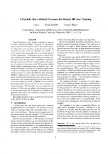
Color histogram of a player (LEFT: white uniform RIGHT: red uniform) Fig. 1. Color histograms: This figure shows two color histograms of selected rectangular regions, each of which is from a different region of the image. The player on left has uniform whose color is the combination of dark blue and white and the player on right has a red uniform. One can clearly see concentrations of color bins due to limited number of colors. In (a) and (b), we set the number of bins, N = 110, where Nh , Ns , and Nv are set to 10.
bt (d) ∈ {1, . . . N } as the bin index associated with the color vector yt (k) at a pixel location d at time t. Figure 1 shows two instances of the color histogram. If we define the candidate region in which we formulate the HSV histogram as R(xt ) , lt + st W , then a kernel density estimate K(xt ) , {k(n; xt )}n=1,...,N of the color distribution at time t is given by [1, 14]: X k(n; xt ) = η δ[bt (d) − n] (1) d∈R(xt )
where δ is the delta function,Pη is a normalizing constant which ensures k to N be a probability distribution, n=1 k(n; xt ) = 1, and a location d could be any pixel location within R(xt ). Eq. (1) defines k(n; xt ) as the probability of a color bin n at time t. If we denote K∗ = {k ∗ (n; x0 )}n=1,...,N as the reference color model and K(xt ) as a candidate color model, then we need to measure the data likelihood (i.e., similarity) between K∗ and K(xt ). As in [1, 14], we apply the Bhattacharyya similarity coefficient to define a distance ξ on HSV histograms. The mathematical formulation of this measure is given by [1]: "
N p X ξ[K , K(xt )] = 1 − k ∗ (n; x0 )k(n; xt ) ∗
n=1
# 21
(2)
Statistical properties of near optimality and scale invariance presented in [1] ensure that the Bhattacharyya coefficient is an appropriate choice of measuring similarity of color histograms. Once we obtain a distance ξ on the HSV color
histograms, we use the following likelihood distribution given by [14]: p(yt |xt ) ∝ e−λξ
2
[K∗ ,K(xt )]
(3)
where λ = 20. λ is suggested in [14, 17], and confirmed also on our experiments. Also, we set the size of bins Nh , Ns , and Nv as 10. The HSV color histogram is a reliable approximation of the color density on the tracked region. However, a better approximation is obtained when we consider the spatial layout of the color distribution. If we define the tracked Pr region as the sum of r sub-regions R(xt ) = R j=1 j (xt ), then we apply the likelihood as the sum of the reference histograms {kj∗ }j=1,...,r associated with each sub-region by [14]: p(yt |xt ) ∝ e
Pr
j=1
−λξ 2 [K∗ j ,Kj (xt )]
(4)
Eq. (4) shows how the spatial layout of the color is incorporated into the data likelihood. In Figure 2, we divide up the tracked regions into two sub-regions in order to use spatial information of the color in the appearance of a hockey player.
Fig. 2. Multi-part color likelihood model: This figure shows our multi-part color likelihood model. We divide our model into two sub-regions and take a color histogram from each sub-region so that we take into account the spatial layout of colors of two sub-regions.
For hockey players, their uniforms usually have a different color on their jacket and their pants and the spatial relationship of different colors becomes important. 2.2
The Filtering Distribution
We denote the state vectors and observation vectors up to time t by x0:t , {x0 . . . xt } and y0:t . Given the observation and transition models, the solution to the filtering problem is given by the following Bayesian recursion [3]: p(yt |xt )p(xt |y0:t−1 ) p(yt |y0:t−1 ) R p(yt |xt ) p(xt |xt−1 )p(xt−1 |y0:t−1 )dxt−1 R = p(yt |xt )p(xt |y0:t−1 ) dxt
p(xt |y0:t ) =
(5)
To deal with multiple targets, we adopt the mixture approach of [17]. The posterior distribution, p(xt |y0:t ), is modelled as an M -component non-parametric mixture model: M X p(xt |y0:t ) = Πj,t pj (xt |y0:t ) (6) j=1
PM
where the mixture weights satisfy m=1 Πm,t = 1. Using the the filtering distribution, pj (xt−1 |y0:t−1 ), computed in the previous step, the predictive distribution becomes M X p(xt |y0:t−1 ) = Πj,t−1 pj (xt |y0:t−1 ) (7) j=1
R
where pj (xt |y0:t−1 ) = p(xt |xt−1 )pj (xt−1 |y0:t−1 )dxt−1 . Hence, the updated posterior mixture takes the form PM
where the new weights (independent of xt ) are given by: " # R Πj,t−1 pj (yt |xt )pj (xt |y0:t−1 ) dxt Πj,t = PM R k=1 Πk,t−1 pk (yt |xt )pk (xt |y0:t−1 ) dxt
Unlike a mixture particle filter by [17], we have M different likelihood distributions, {pj (yt |xt )}j=1...M . When one or more new objects appear in the scene, they are detected by Adaboost and automatically initialized with an observation model. Using a different color-based observation model allows us to track different colored objects.
3
Particle Filtering
In standard particle filtering, we approximate the posterior p(xt |y0:t ) with a Dirac measure using a finite set of N particles {xit }i=1···N . To accomplish this, we sample candidate particles from an appropriate proposal distribution x ˜ it ∼ q(xt |x0:t−1 , y0:t ) (In the simplest scenario, it is set as q(xt |x0:t−1 , y0:t ) = p(xt |xt−1 ),
yielding the bootstrap filter [3]) and weight these particles according to the following importance ratio: i wti = wt−1
We resample the particles using their importance weights to generate an unweighted approximation of p(xt |y0:t ). In the mixture approach of [17], the particles are used to obtain the following approximation of the posterior distribution: p(xt |y1:t ) ≈
M X j=1
Πj,t
X
wti δxit (xt )
i∈Ij
where Ij is the set of indices of the particles belonging to the j-th mixture component. As with many particle filters, the algorithm simply proceeds by sampling from the transition priors (note that this proposal does not use the information in the data) and updating the particles using importance weights derived from equation (8); see Section 3 of [17] for details. In [17], the mixture representation is obtained and maintained using a simple K-means spatial reclustering algorithm. In the following section, we argue that boosting provides a more satisfactory solution to this problem.
4
Boosted Particle Filter
The boosted particle filter introduces two important extensions of the MPF. First, it uses Adaboost in the construction of the proposal distribution. This improves the robustness of the algorithm substantially. It is widely accepted that proposal distributions that incorporate the recent observations (in our case, through the Adaboost detections) outperform naive transition prior proposals considerably [15, 16]. Second, Adaboost provides a mechanism for obtaining and maintaining the mixture representation. This approach is again more powerful than the naive K-means clustering scheme used for this purpose in [17]. In particular, it allows us to detect objects leaving and entering the scene efficiently. 4.1
Adaboost Detection
We adopt the cascaded Adaboost algorithm of Viola and Jones [18], originally developed for detecting faces. In our experiments, a 23 layer cascaded classifier is trained to detect hockey players. In order to train the detector, a total of 6000 figures of hockey players are used. These figures are scaled to have a resolution of 10 × 24 pixels. In order to generate such data in a limited amount of time, we speed the selection process by using a program to extract small regions of the image that most likely contain hockey players. Simply, the program finds regions that are centered on low intensities (i.e., hockey players) and surrounded by high intensities (i.e., rink surface). However, it is important to note that the
data generated by such a simple script is not ideal for training Adaboost, as shown in Figure 3. As a result, our trained Adaboost produces false positives alongside the edge of the rink shown in (c) of Figure 4. More human intervention with a larger training set would lead to better Adaboost results, although failures would still be expected in regions of clutter and overlap. The non-hockey-player subwindows used to train the detector are generated from 100 images manually chosen to contain nothing but the hockey rink and audience. Since our tracker is implemented for tracking hockey scenes, there is no need to include training images from outside the hockey domain.
Fig. 3. Training set of images for hockey players: This figure shows a part of the training data. A total of 6000 different figures of hockey players are used for the training.
The results of using Adaboost in our dataset are shown in Figure 4. Adaboost performs well at detecting the players but often gets confused and leads to many false positives.
(a)
(b)
(c)
Fig. 4. Hockey player detection result: This figure shows results of the Adaboost hockey detector. (a) and (b) shows mostly accurate detections. In (c), there are a set of false positives detected on audience by the rink.
4.2
Incorporating Adaboost in the Proposal Distribution
It is clear from the Adaboost results that they could be improved if we considered the motion models of the players. In particular, by considering plausible motions, the number of false positives could be reduced. For this reason, we incorporate Adaboost in the proposal mechanism of our MPF. The expression for the proposal distribution is given by the following mixture. ∗ qB (xt |x0:t−1 , y1:t ) = αqada (xt |xt−1 , yt ) + (1 − α)p(xt |xt−1 )
(10)
where qada is a Gaussian distribution that we discuss in the subsequent paragraph (See Figure 5). The parameter α can be set dynamically without affecting the convergence of the particle filter (it is only a parameter of the proposal distribution and therefore its influence is corrected in the calculation of the importance weights). When α = 0, our algorithm reduces to the MPF of [17]. By increasing α we place more importance on the Adaboost detections. We can adapt the value of α depending on tracking situations, including cross overs, collisions and occlusions. Note that the Adaboost proposal mechanism depends on the current observation yt . It is, therefore, robust to peaked likelihoods. Still, there is another critical issue to be discussed: determining how close two different proposal distributions need to be for creating their mixture proposal. We can always apply the mixture proposal when qada is overlaid on a transition distribution modeled by autoregressive state dynamics. However, if these two different distributions are not overlapped, there is a distance between the mean of these distributions. If a Monte Carlo estimation of a mixture component by a mixture particle filter overlaps with the nearest cluster given by the Adaboost detection algorithm, we sample from the mixture proposal distribution. If there is no overlap between the Monte Carlo estimation of a mixture particle filter for each mixture component and clusters given by the Adaboost detection, then we set α = 0 so that our proposal distribution takes only a transition distribution of a mixture particle filter.
5
Experiments
This section shows BPF tracking results on hockey players in a digitized video sequence from broadcast television. The experiments are performed using our non-optimized implementation in C on a 2.8 GHz Pentium IV. Figure 6 shows scenes where objects are coming in and out. In this figure, it is important to note that no matter how many objects are in the scene, the mixture representation of BPF is not affected and successfully adapts to the change. For objects coming into the scene, in (a) of the figure, Adaboost quickly detects a new object in the scene within a short time sequence of only two frames. Then BPF immediately assigns particles to an object and starts tracking it. Figure 7 shows the Adaboost detection result in the left column, a frame number in the middle, and BPF tracking results on the right. In Frame 32
q(x)
qada
q*B p( X | X t
t−1)
x
Fig. 5. Mixture of Gaussians for the proposal distribution.
and 33, a small crowd of three players in the middle of the center circle on the rink are not well detected by Adaboost. This is an example of the case in which Adaboost does not work well in clutter. There are only two windows detected by Adaboost. However, BPF successfully tracks three modes in the cluttered environment. Frames 34 and 35 show another case when Adaboost fails. Since Adaboost features are based on different configurations of intensity regions, it is highly sensitive to a drastic increase/decrease of the intensity. The average intensity of the image is clearly changed by a camera flash in Frame 34. The number of Adaboost detections is much smaller in a comparison with the other two consecutive frames. However, even in the case of an Adaboost failure, mixture components are well maintained by BPF, which is also clearly shown in Frame 205 in the figure.
6
Conclusions
We have described an approach to combining the strengths of Adaboost for object detection with those of mixture particle filters for multiple-object tracking. The combination is achieved by forming the proposal distribution for the particle filter from a mixture of the Adaboost detections in the current frame and the dynamic model predicted from the previous time step. The combination of the two approaches leads to fewer failures than either one on its own, as well as addressing both detection and consistent track formation in the same framework. We have experimented with this boosted particle filter in the context of tracking hockey players in video from broadcast television. The results show that most players are successfully detected and tracked, even as players move in and out of the scene. We believe results can be further improved by including
more examples in our Adaboost training data for players that are seen against non-uniform backgrounds. Further improvements could be obtained by dynamic adjustment of the weighting parameter selecting between the Adaboost and dynamic model components of the proposal distribution. Adopting a probabilistic model for target exclusion [11] may also improve our BPF tracking.
7
Acknowledgment
This research is funded by the Institute for Robotics and Intelligent Systems (IRIS) and their support is gratefully acknowledged. The authors would like to specially thank Matthew Brown, Jesse Hoey, and Don Murray from the University of British Columbia for fruitful discussions and helpful comments about the formulation of BPF.
(a) Before a new player appears
(b) 2 frames after
(c) Before two players disappear
(d) 8 frames after
Fig. 6. Objects appearing and disappearing from the scene: This is a demonstration of how well BPF handles objects randomly coming in and out of the scene. (a) and (b) show that a new player that appears in the top left corner of the image is successfully detected and starts to get tracked. (c) and (d) show that two players are disappearing from the scene to left.
32
33
34
35
205 (a) Adaboost detection result
(b) BPF tracking
Fig. 7. BPF tracking result: The results of Adaboost detection are shown on the left, with the corresponding boosted particle filter results on the right.
References 1. Comaniciu, D., Ramesh, V., Meer, P.: Real-Time Tracking of Non-Rigid Objects using Mean Shift. IEEE Conference on Computer Vision and Pattern Recognition, pp. 142-151 (2000) 2. Deutscher, J., Blake, A., Ried, I.: Articulated body motion capture by annealed particle filtering. IEEE Conference on Computer Vision and Pattern Recognition, (2000) 3. Doucet, A., de Freitas, J. F. G., N. J. Gordon, editors: Sequential Monte Carlo Methods in Practice. Springer-Verlag, New York (2001) 4. Freund, Y., Schapire, R. E.: A decision-theoretic generalization of on-line learning and an application to boosting. Computational Learning Theory, pp. 23-37, Springer-Verlag, (1995) 5. Hue, C., Le Cadre, J.-P., P´erez, P.: Tracking Multiple Objects with Particle Filtering. IEEE Transactions on Aerospace and Electronic Systems, 38(3):791-812 (2002) 6. Intille, S. S., Davis, J. W., Bobick, A.F.: Real-Time Closed-World Tracking. IEEE Conference on Computer Vision and Pattern Recognition, pp. 697-703 (1997) 7. Isard, M., MacCormick, J.: BraMBLe: A Bayesian multiple-blob tracker. International Conference on Computer Vision, pp. 34-41(2001) 8. Isard, M., Blake, A.: Condensation – conditional density propagation for visual tracking. International Journal on Computer Vision, 28(1):5-28 (1998) 9. Kalman, R.E.: A New Approach to Linear Filtering and Prediction Problems Transactions of the ASME–Journal of Basic Engineering, vol.82 Series D pp.35-45 (1960) 10. Koller, D., Weber, J., Malik, J.: Robust Multiple Car Tracking with Occlusion Reasoning. European Conference on Computer Vision, pp. 186-196, LNCS 800, Springer-Verlag (1994) 11. MacCormick, J., Blake, A.: A probabilistic exclusion principle for tracking multiple objects. International Conference on Computer Vision, pp. 572-578 (1999) 12. Misu, T., Naemura, M., Wentao Zheng, Izumi, Y., Fukui, K.: Robust Tracking of Soccer Players Based on Data Fusion IEEE 16th International Conference on Pattern Recognition, pp. 556-561 vol.1 (2002) 13. Needham, C. J., Boyle, R. D.: Tracking multiple sports players through occlusion, congestion and scale. British Machine Vision Conference, vol. 1, pp. 93-102 BMVA (2001) 14. P´erez, P., Hue. C, Vermaak, J., Gangnet, M.: Color-Based Probabilistic Tracking. European Conference on Computer Vision, (2002) 15. Rui, Y., Chen, Y.: Better Proposal Distributions: Object Tracking Using Unscented Particle Filter. IEEE Conference on Computer Vision and Pattern Recognition, pp. 786-793 (2001) 16. van der Merwe, R., Doucet, A., de Freitas, J. F. G., Wan, E: The Unscented Particle Filter. Advances in Neural Information Processing Systems, vol. 8 pp 351357 (2000) 17. Vermaak, J., Doucet, A., P´erez, P.: Maintaining Multi-Modality through Mixture Tracking. International Conference on Computer Vision (2003) 18. Viola, P., Jones, M.: Rapid Object Detection using a Boosted Cascade of Simple Features. IEEE Conference on Computer Vision and Pattern Recognition (2001)