JMLR: Workshop and Conference Proceedings 34:49–63, 2014
Proceedings of the 12th ICGI
A bottom-up efficient algorithm learning substitutable languages from positive examples Fran¸ cois Coste Ga¨ elle Garet Jacques Nicolas
[email protected] [email protected] [email protected]
Irisa / Inria Rennes - Bretagne Atlantique Campus universitaire de Beaulieu 35042 Rennes, France
Editors: Alexander Clark, Makoto Kanazawa and Ryo Yoshinaka
Abstract Based on Harris’s substitutability criterion, the recent definitions of classes of substitutable languages have led to interesting polynomial learnability results for expressive formal languages. These classes are also promising for practical applications: in natural language analysis, because definitions have strong linguisitic support, but also in biology for modeling protein families, as suggested in our previous study introducing the class of local substitutable languages. But turning recent theoretical advances into practice badly needs truly practical algorithms. We present here an efficient learning algorithm, motivated by intelligibility and parsing efficiency of the result, which directly reduces the positive sample into a small non-redundant canonical grammar of the target substitutable language. Thanks to this new algorithm, we have been able to extend our experimentation to a complete protein dataset confirming that it is possible to learn grammars on proteins with high specificity and good sensitivity by a generalization based on local substitutability. Keywords: (local) substitutable languages, learning algorithm, canonical grammar, proteins
1. Introduction Based on Harris’s substitutability criterion, the recent definitions of classes of context-free substitutable languages have led to interesting polynomial learnability results for expressive formal languages. These classes are also promising for practical applications: in natural language from the linguistics motivation of the definitions but also in biology to learn grammars modeling protein families, as suggested in our previous study introducing the class of local substitutable languages. To turn theory into practice, we present here an efficient learning algorithm, motivated by intelligibility and parsing efficiency of the result, which directly reduces the positive sample into a small non-redundant canonical grammar of the target substitutable language. We introduce first the definitions of substitutable languages and a first algorithm learning them in section 2, before introducing our algorithm in section 3 and showing its interest experimentally on artificial and applicative datasets in section 4.
c 2014 F. Coste, G. Garet & J. Nicolas.
Coste Garet Nicolas
2. Learning substitutable languages 2.1. Formal languages and substitutability We introduce briefly here the definitions and notations related to substitutable languages. Let Σ be a non-empty finite set of atomic symbols. Σ∗ is the set of all finite strings over the alphabet Σ. We denote the length of a string x by |x|, the empty string by λ, the set of non-empty strings Σ∗ \ {λ} by Σ+ and the set of strings of length k {x : |x| = k} by Σk . For a language L ⊆ Σ∗ , the set of its substrings is Sub(L) = {y ∈ Σ∗ : x, z ∈ Σ∗ , xyz ∈ L} and the set of its contexts is Con(L) = {hx, zi ∈ Σ∗ × Σ∗ : y ∈ Σ∗ , xyz ∈ L}. The empty context is hλ, λi. The distribution of a string y ∈ Σ∗ with respect to a language L is defined to be its set of contexts in L: DL (y) = {hx, zi ∈ Σ∗ × Σ∗ : xyz ∈ L}. Two strings y1 and y2 in Σ∗ are syntactically congruent for a language L, denoted y1 ≡L y2 , iff DL (y1 ) = DL (y2 ). The equivalence relation ≡L defines a congruence on the monoid Σ∗ since straightforwardly y1 ≡L y2 implies ∀x, z in Σ∗ , xy1 z ≡L xy2 z. We denote the congruence class of y by [y]L = {y 0 ∈ Σ∗ : y ≡L y 0 } and the concatenation of two languages L1 and L2 by L1 L2 = {y1 y2 : y1 ∈ L1 , y2 ∈ L2 }. The congruence class [λ] is called the unit congruence class. The set {y : DL (y) = ∅} = Σ∗ \Sub(L), when non-empty, is called the zero congruence class. A congruence class is non-zero if it is a subset of Sub(L). Note that for any strings y1 , y2 in Σ∗ , [y1 y2 ]L ⊇ [y1 ]L [y2 ]L . Interested by learnability of natural languages and inspired by distributional learning, Clark and Eyraud (2007) introduced the substitutable languages as a simple formal class of languages based on Harris’s substitutability criterion. Two non-empty strings y1 and . y2 are said to be weakly substitutable in a language L, denoted y1 =L y2 , iff there exists x, z ∈ Σ∗ , such that xy1 z ∈ L ∧ xy2 z ∈ L. Substitutable languages are those such that weak . substitutability implies syntactic congruence, i.e. such that y1 =L y2 implies y1 ≡L y2 (or equivalently, such that DL (y1 ) ∩ DL (y2 ) 6= ∅ implies DL (y1 ) = DL (y2 )). At the word level, we get the following definition: Definition 1 (Clark and Eyraud, 2007) A language L is substitutable iff for any x1 , y1 , z1 , x2 , y2 , z2 ∈ Σ∗ , y1 , y2 6= λ : x1 y1 z1 ∈ L ∧ x1 y2 z1 ∈ L ⇒ (x2 y1 z2 ∈ L ⇔ x2 y2 z2 ∈ L). Carrying on an analogy between substitutability for context-free languages and reversibility introduced by Angluin (1982) for regular languages, Yoshinaka (2008) introduced the hierarchy of k, l-substitutable context-free language as the counterpart of the k-reversible hierarchy for regular languages. In this hierarchy, expressiveness increases with the parameters k and l by restricting substitutability to occur only in same right and left contexts of respective length k and l. Just as for substitutable languages, one can define two non-empty strings y1 and y2 to be weakly k, l-substitutable in context hu, vi ∈ Σk × Σl in a language . L, denoted uy1 v =L uy2 v, iff there exists x, z ∈ Σ∗ , such that xuy1 vz ∈ L ∧ xuy2 vz ∈ L. The k, l-substitutable languages are those such that weak substitutability in a context from . Σk × Σl implies syntactic congruence in the same context, i.e. such that uy1 v =L uy2 v implies uy1 v ≡L uy2 v (or equivalently, such that DL (uy1 v)∩DL (uy2 v) 6= ∅ implies DL (uy1 v) = DL (uy2 v)):
50
Efficient algorithm learning substitutable languages from positive examples
Definition 2 (Yoshinaka, 2008) A language L is k, l-substitutable iff for any x1 , y1 , z1 , x2 , y2 , z2 ∈ Σ∗ , u ∈ Σk , v ∈ Σl , uy1 v, uy2 v 6= λ : x1 uy1 vz1 ∈ L ∧ x1 uy2 vz1 ∈ L ⇒ (x2 uy1 vz2 ∈ L ⇔ x2 uy2 vz2 ∈ L). The definition of the substitutable strings y1 and y2 above are based on common global contexts. In Coste et al. (2012), we introduced for the characterization of proteins a less stringent criterion based on common local contexts that applies to more practical cases. Introducing the parameters k and l to set the minimal length of the left and right local contexts, two non-empty strings y1 and y2 are said weakly (k, l)-local substitutable in a . ∗ k l language L, denoted y1 =k,l L y2 , iff there exists x1 , x2 , z1 , z2 ∈ Σ ,u ∈ Σ , v ∈ Σ , such that: x1 uy1 vz1 ∈ L ∧ x2 uy2 vz2 ∈ L. The k, l-local substitutable languages are those such . that weak (k, l)-local substitutability implies syntactic congruence, i.e. such that y1 =k,l L y2 k,l k l implies y1 ≡L y2 (or equivalently if we define DL (y) as {hu, vi ∈ Σ × Σ : uyv ∈ Sub(L)}, k,l k,l such that DL (y1 ) ∩ DL (y2 ) 6= ∅ implies DL (y1 ) = DL (y2 )): Definition 3 (Coste et al., 2012) A language L is k, l-local substitutable iff for any x1 , y1 , z1 , x2 , y2 , z2 , x3 , z3 ∈ Σ∗ , u ∈ Σk , v ∈ Σl , uy1 v, uy2 v 6= λ : x1 uy1 vz1 ∈ L ∧ x3 uy2 vz3 ∈ L ⇒ (x2 y1 z2 ∈ L ⇔ x2 y2 z2 ∈ L). And by crossing the local extension with the extension by Yoshinaka (2008), we get the definition of the k, l-local contextually substitutable languages: Definition 4 (Coste et al., 2012) A language L is k, l-local contextually substitutable iff for any x1 , y1 , z1 , x2 , y2 , z2 , x3 , z3 ∈ Σ∗ , u ∈ Σk , v ∈ Σl , uy1 v, uy2 v 6= λ : x1 uy1 vz1 ∈ L ∧ x3 uy2 vz3 ∈ L ⇒ (x2 uy1 vz2 ∈ L ⇔ x2 uy2 vz2 ∈ L). The class of substitutable languages defined by Clark and Eyraud (2007) stands at the limit of the hierarchy of k, l-local substitutable languages when k and l tend to infinity, and conversely is the first class in the hierarchy of k, l-substitutable languages, with k and l equal to 0. As for reversible languages, we will thus use the term zero-substitutable language when we want to designate specifically this class and we will keep substitutable languages as a generic term for the classes of languages formally defined with respect to a substitutability criterion. In the next sections, we will consider the problem of learning substitutable languages with algorithms using context-free grammar representations. A context-free grammar is defined classically as a quadruple G = hΣ, N, S, P i where Σ is a finite alphabet of terminal symbols, N is a finite alphabet of variables or non-terminals, S ∈ N is the start symbol and P is a finite set of production rules of the form N × (N ∪ Σ)+ . We say that a sequence δAγ from (N ∪ Σ)+ can be derived into δαγ, denoted δAγ ⇒G δαγ if there exists a production + rule A → α in P . The transitive closure of ⇒G is denoted ⇒G and its reflexive transitive ∗ closure ⇒G . The set of strings that can be derived from S is the set of sentential forms ∗ {α ∈ (N ∪ Σ)∗ : S ⇒G α} and the context-free language defined by a context-free grammar G is the set of sentential forms consisting entirely of terminal symbols L(G) = {w ∈ Σ∗ : ∗ S ⇒G w}. Let us note that from our definition of production rules, the empty string cannot be derived from G. In that case, a context-free grammar G is in Chomsky Normal Form (CNF) iff its productions are of the form A → BC, A → a, where A, B, C ∈ N and a ∈ Σ. 51
Coste Garet Nicolas
2.2. A first grammatical inference algorithm for substitutable languages For our experiments on grammatical inference of k, l-local substitutable languages in Coste et al. (2012), we implemented the algorithm 1 that is a straightforward adaptation of the SGL algorithm introduced for substitutable languages by Clark and Eyraud (2007). Algorithm 1: SGLLS (Substitution Graph Learner for k, l-local substitutable languages)
1 2
3 4
5 6 7
8 9
10 11
12
13
14
Input: Set of sequences K on alphabet Σ, int k, int l Output: Grammar G = hΣ, NK , SK , PK i /* Partition Sub(K) in substitutability classes */ CK ← Local substitutability classes(K, k, l) ∀y ∈ Sub(K), CK (y) = C ∈ CK : y ∈ C /* Build grammar */ NK ← ∅, PK ← ∅ for C ∈ CK do /* A non-terminal for each substitutability class */ NK ← NK ∪ {JCK} if C ∩ K 6= ∅ then SK ← JCK
/* Productions rules for each substring in the class */ for y ∈ C do if |y| > 1 then /* Branching rules: a ’CNF’ rule for each split */ for y1 ∈ Σ+ , y2 ∈ Σ+ : y1 y2 = y do PK ← PK ∪ {JCK → JCK (y1 )KJCK (y2 )K} else /* Terminal rule */ PK ← PK ∪ {JCK → y}
return hΣ, NK , SK , PK i
Algorithm 2: Local substitutability classes
1 2
3
Input: Set of sequences K on alphabet Σ, int k, int l Output: k, l local substitutability classes on K /* Build substitutability graph on substrings */ V ← {y ∈ Σ+ : y ∈ Sub(K)} E ← {{y1 , y2 } ∈ V × V : uy1 v ∈ Sub(K), uy2 v ∈ Sub(K), y1 6= y2 , u ∈ Σk , v ∈ Σl } /* Return connected components of graph */ return Connected components(hV, Ei)
Given a set of sequences K and parameters k and l specifying the target class of local substitutable languages, this algorithm partitions all the substrings of K into k, l-local substitutability classes in K using a substitution graph and returns a CNF context-free grammar. This grammar contains a non-terminal symbol JCK for each substitutability class C, branching rules, carrying on the generalization, JCK (y1 y2 )K → JCK (y1 )KJCK (y2 )K for 52
Efficient algorithm learning substitutable languages from positive examples
each possible concatenation y1 y2 that results in a substring of K — where CK (x) identifies the substitutability class of x — and terminal rules that generate terminal symbols. Let us remark that this algorithm may be adapted to other classes of substitutable languages, simply by changing the function returning the substitutability classes. This can be achieved by modifying in line 2 of algorithm 2 the substrings in relation in the substitution graph. The definition of the set of edges was replaced for substitutable languages by: E ← {{y1 , y2 } ∈ V × V : xy1 z ∈ K, xy2 z ∈ K, y1 6= y2 , x ∈ Σ∗ , z ∈ Σ∗ }, for k, l-substitutable languages by: E ← {{uy1 v, uy2 v} ∈ V × V : xuy1 vz ∈ K, xuy2 vz ∈ K, y1 6= y2 , x ∈ Σ∗ , z ∈ Σ∗ , u ∈ Σk , v ∈ Σl } and for k, l-local context substitutable languages by: E ← {{uy1 v, uy2 v} ∈ V × V : uy1 v ∈ Sub(K), uy2 v ∈ Sub(K), y1 6= y2 , u ∈ Σk , v ∈ Σl }. This can be done in all the algorithms presented in this paper and we can thus restrict ourselves hereafter to the k, l-local substitutability case to simplify the presentation without loss of generality. Even if it does not always return a grammar from the target class of languages, this kind of algorithm enables to identify a target grammar G in polynomial time from a characteristic sample of polynomial size in |G|.τG , where τG is the thickness of the grammar, provided that its context-free substitutability class is known (Clark and Eyraud, 2007; Yoshinaka, 2008). But even if the algorithm is polynomial, it cannot be used in practice on real data sets as witnessed by our first experiments on proteins (Coste et al., 2012), since it requires hours for each run of the algorithm preventing significant cross-validation and more systematic studies on the parameters’ influence. As a matter of fact, the resulting grammars suffer from embedding too many ambiguities and redundancies. From a parsing perspective or even with the simple goal of manually checking and interpreting the rules, the obtained grammars are too large, an issue that affects also clearly the learning run time. Hence, motivated by speeding up the experiments and driven by legibility and parsing efficiency of the grammar, we have designed a new algorithm, implemented in Fall 2012 but still unpublished, learning directly grammars in a minimal non-redundant form. The next section describes this new algorithm.
3. Learning reduced grammars 3.1. Reduced Grammars To improve parsing time and improve the legibility of grammars learnt by SGLLS as well as their derivation trees, the Chomsky Normal Form can be transformed into a reduced form that avoids unnecessary derivation steps and redundancies by: • removing unnecessary non-terminals whose derivation is deterministic(if a non-terminal A is the left-hand side of only one rule A → α, the non-terminal and the rule are deleted and each occurrence of A in the other rules is replaced by α); • minimizing the right-hand sides of the production rules (replacing any substring β of the right-hand side by the smallest substrings α in N ∪ Σ from which β can be derived) The first reduction corresponds to removing non-terminals that give rise to vacuous local derivation trees (Clark, 2011). We called this kind of congruence classes composite since they can be factorized into the concatenation of a set of congruence classes. Formally: 53
Coste Garet Nicolas
Definition 5 (Composite congruence class) Let a language L whose set of non-zero and non-unit congruence classes is C + . A class [y] ∈ C + is composite for L iff: ∃[x1 ], . . . [xm ] ∈ C + , m ≥ 2, [y] = [x1 ] . . . [xm ] A congruence class is prime if it is not composite. These classes are the ones to be kept as non-terminals. In the algorithms, we use a more operational characterization of prime (and composite) congruence classes which can be deduced from syntactic congruence properties: Lemma 6 Let a language L whose set of non-zero and non-unit congruence classes is C + . A class [y] in C + is prime for L iff ∀y1 y2 ∈ [y], [y] 6⊂ [y1 ][y2 ]. Proof This is a simple application of the fact that the contexts of a string include the concatenation of its substring contexts. Any equation involving m > 2 substrings is thus superseded by the equation involving only the first substring and the concatenation of the other substrings. Moreover, the equation can be replaced by an inclusion since the other direction is already granted. The second reduction, since non-terminals and the languages they generate are fixed, can be handled as an extension of minimal grammar parsing (Carrascosa et al., 2011): each non-terminal generates a whole set of substitutable words rather than a single word. It can be solved similarly by dynamic programming on graphs representing right-hand side’s strings of the rules, with the added difficulty that all non-redundant paths have to be found. Solving this problem is equivalent to searching for each right-hand side α the set of non-redundant strings generating all the sequences generated from α (see next section for details). Note that this algorithm results in the same set of rules than the algorithm recently proposed by Clark (2014) even if approaches differ: building directly the set of non-redundant rules by dynamic programming in our case versus filtering out from the whole set of potential valid rules the so-called pleonastic rules. Based on the ‘fundamental lemma’ of substitutable languages proven by Clark (2014), the reduced form computed by this algorithm is thus also a canonical form of the grammar for substitutable languages. So far we have only discussed the reduction of the grammar into a minimal nonredundant canonical form. We present in the next section the algorithm ReGLiS based on the same dynamic programming ideas but learning simultaneously this reduced form and the content of the substitutability classes by a bottom-up reduction of the sample. 3.2. Learning reduced grammars: ReGLiS The ReGLiS algorithm is detailed in algorithm 3. Taking as input a sample of strings K on an alphabet Σ, and two parameters k and l defining the target class of local substitutable languages, ReGLiS returns a grammar in reduced form of the target language when K includes a characteristic sample of the language for SGLLS . Like SGLLS presented in section 2.2, ReGLiS builds a grammar based on a set of equivalence classes CK defined from weak substitutability evidence in K. Let us remark that the rest of the algorithm is independent from the actual targeted class of languages: 54
Efficient algorithm learning substitutable languages from positive examples
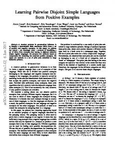
the classes are based here on k, l-local substitutability, but other weak substitutability criteria can be used to adapt the algorithm to other classes of substitutable languages. In contrast with SGLLS introducing a non-terminal for each equivalence class, ReGLiS takes care to introduce a non-terminal only for the substitutability classes containing more than one string and satisfying Lemma 6 on CK which we call K-prime substitutability classes. The symbol introduced for the K-prime substitutability class containing K is the start symbol. For each of these non-terminals, the set of production rules contains as many rules as strings in its substitutability class, deriving each in one step the non-terminal into one of these strings. The grammar built this way is only able to generate the strings from K and contains also unreachable rules linking each non-terminal with the substrings of its substitutability class. A generalization step at the core of the algorithm is then achieved by a bottom-up rewriting process on the right-hand sides, starting by the shortest ones and optimizing the set of branching rules by dynamic programming on a parsing graph for each right-hand side of rule. N1
0
a
1
b
2
c
N3
N2
3
d
4
e
5
N4
Figure 1: Example of parsing graph for abcde: non-redundant right-hand sides are aN1 e and N3 N2 .
Specifically, for each right-hand side α, a parsing graph is built by algorithm 4 (see example in figure 1). Intuitively, the graph represents all the possible generation of substrings from α by substitutability class non-terminals. Finding all non-redundant most general right-hand sides allowing to generate α, is done by algorithm 5. Forgetting the symbols, this algorithm focuses on paths in the parsing graph. Paths are represented as sequences of vertices, and adding a vertex i at the end of a path π is denoted by the concatenation π.i. A path π2 = t1 . . . tm is reducible in π = s1 . . . sn , denoted π ≺r π2 , if π is a strict substring of π2 that has the same beginning and end than π2 , i.e. s1 = t1 and sn = tm . A path π is said irreducible if it is minimal for the partial order ≺r . Algorithm 5 implements a dynamic programming search of all irreducible paths in the parsing graph and return then all the non-redundant right-hand side generalizing α to be used to replace it. Two improvements have been included in the algorithm to enable also the identification of the target language for some samples on which SGLLS would not succeed. First, if during the reduction one gets an already existing right-hand side in the set of production rules, the corresponding non-terminals are unified to avoid generating the same substring by two different non-terminals and still ensure the transitivity of the substitution classes. Second, since languages recognized by non-terminals are increasing, new edges can appear in the
55
Coste Garet Nicolas
parsing graph despite the ordering of the right-hand sides. In such cases, optimization has to be performed again. The loop around the optimization ensures its convergence and may then require less examples to build the target grammar than SGLLS . Algorithm 3: ReGLiS
1
2 3
4 5 6 7 8
9
10 11 12
13 14
15 16 17 18 19 20
21 22
(Learning Reduced Grammar by k, l-Local Substitutability)
Input: Set of sequences K on alphabet Σ, int k, int l Output: Grammar G = hΣ, NK , SK , PK i /* Partition Sub(K) in substitutability classes */ CK ← Local substitutability classes(K, k, l) /* Non-terminals for K-primes and their productions in Sub(K) */ NK ← ∅, PK ← ∅ for C ∈ CK do /* Start symbol */ if C ∩ K 6= ∅ then NK ← NK ∪ {JCK} SK ← JCK for y ∈ C do PK ← PK ∪ {JCK → y} /* Non-terminal symbols for K-prime substitutability classes */ else if (|C| > 1) and (6 ∃C 0 ∈ CK : ∀y ∈ C, ∃y 0 ∈ C 0 , ∃v ∈ Σ+ , y = y 0 v) and (6 ∃C 0 ∈ CK : ∀y ∈ C, ∃y 0 ∈ C 0 , ∃u ∈ Σ+ , y = uy 0 ) then NK ← NK ∪ {JCK} for y ∈ C do PK ← PK ∪ {JCK → y} /* Generalization */ repeat P ← PK ; PK ← ∅ /* Branching rules */ for (JCK → α) ∈ P ordered by increasing |α| do P G ← Build parsing graph(α, P ) for β ∈ Non redundant rhs(P G) do if ∃(JC 0 K → β) ∈ Pk , JC 0 K 6= JCK then Unify(JC 0 K, JCK, PK ) PK ← PK ∪ (JCK → β)
until PK = P return hΣ, NK , SK , PK i
3.3. Complexity of ReGLiS algorithm Let K be a training sample of size |K| and n be the size of its longest sequence. The complexity of the algorithm 3 is determined by three critical parts: line 3 The creation of the local substitutability classes, which depends on the number of substrings in Sub(K). This number is a main parameter for the rest of the algorithm since all operations are working on the elements of Sub(K).
56
Efficient algorithm learning substitutable languages from positive examples
Algorithm 4: Build parsing graph
1 2 3 4 5 6
7
Input: Sequence α, Set of rules P Output: Parsing graph hV, Ei V ← {i ∈ [0, |α|]} /* vertices */ E ← ∅ /* labeled directed edges */ for i ∈ V do for j ∈ V : i < j and (i, j) 6= (0, |α|) do if ∃(JCK → α[i + 1, j]) ∈ P then E ← E ∪ (i, j, JCK) return hV, Ei
Algorithm 5: N on redundant rhs
1 2 3
4 5 6 7 8 9 10 11
Input: Parsing graph: hV, Ei Output: Set of non-redundant right-hand side from parsing graph: R R←∅ paths[0] ← {{0}} for i ← 1 to |V | do /* memorize the set of irreducible paths arriving in i */ S P ← (j,i,l)∈E (paths[j].i) paths[i] ← {x ∈ P : 6 ∃y ∈ P, y ≺r x} for path ∈ paths[n] do rhs ← λ for i ← 1 to |path| do rhs ← rhs.βi with βi : (path[i − 1], path[i], βi ) ∈ E R ← R ∪ rhs return R
line 9 The reduction of the number of classes, which reduces the number of substrings to be considered in the next part of the algorithm. line 16 The minimization of the grammar, which includes the creation of parsing graphs as the main source of complexity. It is easy to see that the complexity of this part depends on the number of rules in the grammar. Building local substitutability classes Complexity of Local substitutability classes depends on the number of elements in Sub(K). Indeed, the algorithm starts building the substitutability graph (the graph of shared contexts) by creating a vertex for each prefix of the suffix at each position of each sequence (i.e. creating the set of substrings Sub(K)). During this loop, a table T giving for each context its set of substrings is created. For a sequence of length m, the maximal number of substrings created in CK and in T is m(m + 1)/2. Since n is the size of the longest sequence in K, the total number of substring occurrences is O(|K|n2 ). The goal then is to find the maximally connected components of the substitutability graph. By definition, each entry in table T points to a connected component. Instead of creating the whole substitutability graph, it is sufficient to create a chain for all set of 57
Coste Garet Nicolas
substrings in table T . The resulting graph contains the same connected components than the whole graph and the complexity remains in O(|K|n2 ). Note that the class CK (x) of each substring x can be stored during the search of connected components. Reduction of the number of classes In the loop line 3–12, each element (connected component) of CK is visited once, so the interior loops are performed O(|K|n2 ) times. Globally, the line 9 visits all substrings once (O(|K|n2 )), and for each substring, all its prefixes and suffixes (O(2n)). Each substring is visited only once globally because it appears in only one connected component. The treatment of each substring in each class involves an intersection of all its prefixes with other prefixes of other substrings in the same class, an operation linear with respect to the number of prefixes, i.e. O(n). So the global complexity of this loop is O(n3 ). This loop reduces in practice the number of classes and the number of substrings that belong to a substitutability class. The new set of available substrings is denoted K −P rime. Generalization and minimization of the grammar In this part, (line 13 to 21), the main loop is repeated until no more right-hand side α of the grammar rules can be reduced. The worst case for this loop occurs when all substrings of length ≤ l, l = 1 . . . n are considered in turn for the reduction of α. Thus, the maximal number of steps for the loop is n. The complexity of the interior loop (line 15 to 20) is bounded by the number of righthand sides of the grammar A = {α | X → α ∈ PK } and their length since the loop considers all α substrings for the parsing graphs. If t denotes the size of the target grammar (number of rules × size of rules), then the worst case complexity of generalization and minimization is O(n.t). The overall complexity of the algorithm is then O(max(n3 , n.t)). The rest of the paragraph further investigates this complexity to remove the dependence to the size t of the target grammar in the formula. Initially, the number of rules is bounded by |K − P rime| and the length of α is O(n). So the first step is bounded in O(|K − P rime|n). The number of rules can increase at each step of the loop, but if so, the length of the new rules decreases. If no substring is removed during the first step of the algorithm (|K − P rime| = |Sub(K)|), the worst case is to get |A| = 2n−1 rules in the target grammar (Chomsky Normal Form). It occurs when each rule can be split into 2 parts at each position of α, giving rise to the maximum number of irreducible paths in the parsing graph. If some substrings are removed, the number of irreducible paths can only decrease. For each sequence si of K, there exists a decomposition si = u1 v1 u2 v2 . . . up such that each uj , j ∈ [1, p], is a substring belonging to a prime class (prime substring), each vj , j ∈ [1, p − 1], is a substring that is not prime and mi = |v1 | + |v2 | + . . . + |vp−1 | is maximum. The number of decompositions of si is the product of the number of decompositions of primes since non-prime substrings have a single decomposition. At worst this leads to 2n−mi possibilities. For the whole training sample, the complexity of the generalization and minimization of the grammar, and thus of the whole algorithm, can thus reach O(2n−mini (mi ) ), being dominated by the theoretical bound for the target grammar size t. 58
Efficient algorithm learning substitutable languages from positive examples
4. Experiments 4.1. Comparison of run times on simulated data We have first launched some tests on simulated data sets to compare the practical complexity of the new algorithm introduced in this paper with respect to the algorithm used in Coste et al. (2012). The run time gain has been estimated on training samples with increasing number and increasing length of strings which were randomly generated to resemble those encountered for the protein classification task in Coste et al. (2012). For the first experiment, a random string of length 20 on a 40 symbols alphabet was randomly generated and sorted according to an arbitrary order on the alphabet to group sequentially identical characters as if it was the result of recoding a protein sequence with respect to blocks of a partial multiple sequence alignment (Coste et al., 2012; Kerbellec, 2008). To obtain a target number of similar strings, new strings were iteratively generated by replacing each character of the last generated string with a probability of 25% into a random symbol of the alphabet and by sorting the string. To study the importance of the length, the same generation procedure was used but with the number of strings set to 20 and the alphabet size set to twice the length of the sequences in the sample, this latter value coming from observation of practical protein experiments. Results presented in figure 2 show that there is an obvious advantage in time when the number of strings increase. The length parameter has a high impact on the run time as it was expected in the complexity analysis. The curve shows that for a given amount of resource, the new algorithm allows a shift of about 10 in the length of strings, a difference that may be of high importance in practice. 600
350
ReGLiS SGLLS
time (seconds)
time (seconds)
250
400
300
200
200 150 100
100
0
ReGLiS SGLLS
300
500
50
20
40
60
80
100
120
0
140
number of strings
5
10
15
20
25
30
length of strings
(a) function of the number of strings (b) function of the length of strings in in the training sample the training sample Figure 2: Run time comparison between old and new learning algorithms implementations
In figure 3, run times for the two main parts of the algorithm, the detection of prime classes and the reduction of the grammar, have been extracted from the total. As expected, the complexity is determined by the reduction part and grows exponentially in function of the length of strings in the training set.The detection of prime classes seems to stay linear, an empirical behavior better than the theoretical worst case complexity.
59
Coste Garet Nicolas
30
200
detection of prime classes reduction of grammar total
25
detection of prime classes reduction of grammar total
time (seconds)
time (seconds)
150 20
15
10
100
50 5
0
20
40
60
80
100
120
0
140
number of strings
5
10
15
20
25
30
length of strings
(a) function of the number of strings (b) function of the length of strings in in the training sample the training sample Figure 3: Run time for K-prime classes detection, grammar reduction and whole algorithm
4.2. Application to protein families Motivated by the characterization of functional families of Algae enzymes (Coste et al., 2014), we aim at learning characteristic context-free grammar signatures of protein families which capture long distance sequential dependencies. In Coste et al. (2012), we show the interest of using local substitutability on a small protein dataset extracted from Dyrka and Nebel (2009). With our new learning algorithm, it becomes then possible to run more demanding tests. By way of illustration, when our implementation of SGLLS for Coste et al. (2012) required almost a day, our Python implementation of ReGLiS takes only a few minutes for one experiment. We have then been able to complete our experimentation on the whole dataset from Dyrka and Nebel (2009) and we present the results in Table 1. 1 In all these experiments, we use a 10-fold cross validation and choose relatively small k and l parameters since learning occurs on block strings that are an order of magnitude shorter than amino acids sequences. A reasonable assumption is that some a priori knowledge may exist on the length of relevant contexts in the target application. In the case of proteins, small contexts are expected since interactions concerns few amino-acids. Practical values range from 3 to 7. In all cases, one should avoid higher values since it comes down to using (global) substitutability. Note that we have not made extensive tests on this issue and it is certainly a valuable research track. Overall, it can be observed that local substitutability, using well chosen k and l values, significantly improves the recall with respect to global substitutability, without losing precision. Stochastic grammars get better results in terms of F-measure, except if precision is fixed to a high level. In such a case the recall obtained by ReGLiS is usually better. It is desirable to obtain a high specificity because biological experiments on proteins are expensive and a limited set of candidates can be evaluated and validated in practice. When possible, we also compared our results with results obtained using Prosite regular expressions built on the basis of expert-provided multiple alignments of subsequences of these families. The Prosite patterns span generally around 10 positions whereas the whole protein is about 300 letters long. In consequence, such a pattern has a good recall but weak 1. Details of experiments and results are available at http://www.irisa.fr/dyliss/reglis
60
Efficient algorithm learning substitutable languages from positive examples
precision due to its generality. In contrast, our method takes into account whole sequences. The corresponding grammar has thus a high specificity. The interesting point is that despite their specificity, the level of recall obtained by the grammars appears to remain relatively high, our best recall results being comparable to those of the Prosite’s patterns built by experts. Hence, although the method can still be refined by grammar weighting schemes, this study confirms that local substitutability can be considered as a promising and effective criterion for sequence generalization, especially for the cases requiring an excellent precision.
Substitutable 3,3-Local substitutable 4,4-Local substitutable 5,5-Local substitutable 6,6-Local substitutable 7,7-Local substitutable Stochastic CFG Dyrka and Nebel (2009)
Precision 1 1 1 1 1 1 1 0.15 0.75
Zinc finger Recall F-measure 0.1 0.36 0.2 0.33 0.25 0.4 0.33 0.5 0.5 0.67 0.55 0.7 0.1 0.18 1 0.26 0.87 0.85
Precision 1 1 1 1 1 1 1 0.5 0.98
MPI phos. Recall F-measure 0.15 0.26 0.5 0.67 0.6 0.75 0.67 0.8 0.62 0.77 0.53 0.69 0.3 0.46 1 0.67 0.89 0.93
Substitutable 3,3-Local substitutable 4,4-Local substitutable 5,5-Local substitutable 6,6-Local substitutable 7,7-Local substitutable Prosite Stochastic CFG Dyrka and Nebel (2009)
Precision 1 1 1 1 1 1 1 1
PS00219 Recall F-measure 0.2 0.33 0.72 0.84 0.7 0.82 0.68 0.8 0.6 0.75 0.5 0.67 0.6 0.75 1 1
Precision 1 1 1 1 1 1 1 1 0.1 0.79
PS00063 Recall F-measure 0.23 0.37 0.58 0.73 0.6 0.75 0.66 0.8 0.7 0.82 0.65 0.79 0.8 0.89 0.05 0.1 1 0.18 0.65 0.71
Table 1: Sequence class prediction by grammars obtained for different families with 10-fold cross-validation
Conclusion With ReGLiS we have proposed another step, after the introduction of local substitutable languages, towards practical applications of substitutable language learning. To continue in this direction, on the theoretical side, we would like to better characterize the learnability gain provided by ReGLiS compared to SGL and, on the practical side, we would like to better understand the scope of substitutability criteria for applications and derive datadriven heuristic choices of substitutability classes.
Acknowledgments This work benefited from the support of the French Government run by the National Research Agency and with regards to the investment expenditure programme IDEALG ANR10-BTBR-04. GG is funded by French ‘Region Bretagne’ grant ARED ENZYME No. 6958. 61
Coste Garet Nicolas
References D. Angluin. Inference of reversible languages. J. ACM, 29(3):741–765, 1982. R. Carrascosa, F. Coste, M. Gall´e, and G. G. Infante L´opez. The smallest grammar problem as constituents choice and minimal grammar parsing. Algorithms, 4(4):262–284, 2011. A. Clark. A language theoretic approach to syntactic structure. In M. Kanazawa, A. Kornai, M. Kracht, and H. Seki, editors, The Mathematics of Language, volume 6878 of Lecture Notes in Computer Science, pages 39–56. Springer Berlin Heidelberg, 2011. A. Clark. Learning trees from strings: A strong learning algorithm for some context-free grammars. Journal of Machine Learning Research, 14:3537–3559, 2014. A. Clark and R. Eyraud. Polynomial identification in the limit of substitutable context-free languages. Journal of Machine Learning Research, 8:1725–1745, August 2007. F. Coste, G. Garet, and J. Nicolas. Local Substitutability for Sequence Generalization. In Jeffrey Heinz, Colin de la Higuera, and Tim Oates, editors, ICGI 2012, volume 21 ´ of JMLR Workshop and Conference Proceedings, pages 97–111, Washington, Etats-Unis, Sep 2012. MIT Press. F. Coste, G. Garet, A. Groisillier, J. Nicolas, and T. Tonon. Automated enzyme classification by formal concept analysis. In C. Vera Glodeanu, M. Kaytoue, and C. Sacarea, editors, ICFCA, volume 8478 of Lecture Notes in Computer Science, pages 235–250. Springer, 2014. ISBN 978-3-319-07247-0. W. Dyrka and J.-C. Nebel. A stochastic context free grammar based framework for analysis of protein sequences. BMC Bioinformatics, 10(1):323+, October 2009. G. Kerbellec. Apprentissage d’automates mod´elisant des familles de s´equences prot´eiques. PhD thesis, Universit´e Rennes 1, 2008. R. Yoshinaka. Identification in the limit of (k,l)-substitutable context-free languages. In Proceedings of the 9th international colloquium conference on Grammatical inference: theoretical results and applications, ICGI’08, pages 266–279, 2008.
Appendix A. Example of reduction of grammar on natural language In this appendix, we illustrate the interest of the prime classes and the reduced grammar form on the following training set K:
K ={”Major General was here yesterday morning.”, ”Major General went here yesterday morning.”, ”Major General will be there tomorrow morning.”, ”He will be gone tomorrow evening.”}
62
Efficient algorithm learning substitutable languages from positive examples
Then the grammar obtained by the classical approach introducing a non-terminal for each substitutability class and splitting the rules in all possible rules in Chomsky normal form would be: X47 →0 yesterday 0
X1 → X2 X29 |X19 X16 |X5 X15 |X19 X41 |X35 X15
X46 → X3 X43 |X11 X19 |X23 X13
X6 →0 was0 |0 went0
X45 → X20 X2
X4 → X13 X42
X44 → X20 X1 |X45 X29 |X34 X16 |X9 X15
X5 → X2 X4 |X19 X42
X43 → X20 X19 |X45 X13
X32 → X27 X17 |X28 X15
X42 →0 tomorrow0
X33 → X21 X9 |X39 X5 |X8 X4 |X40 X42
X41 → X42 X15
X30 → General
X40 → X30 X46 |X21 X43 |X39 X19 |X25 X13 |X21 X34 |X8 X13 S → X30 X24 |X21 X31 |X10 X32 |X36 X17 |X26 X15 |X39 X1 |X25 X29 |X40 X41 |X21 X44 |X8 X29 |X40 X16 |X33 X15
X31 → X6 X32 |X22 X17 |X12 X15 |X20 X1 |X45 X29 |X43 X41 X36 → X30 X37 |X21 X22 |X10 X27 X37 → X3 X22 |X18 X27
X29 → X13 X16 |X4 X15 |X13 X41 |X38 X15
X34 → X20 X19 |X45 X13
X28 → X27 X47
X35 → X2 X38 |X19 X42
X25 → X30 X23 |X21 X45 |X39 X2
X38 → X13 X42
X24 → X3 X31 |X18 X32 |X37 X17 |X14 X15 |X11 X1 |X23 X29 |X46 X41
X39 → X30 X11 |X21 X20
X27 →0 here0
X18 → X3 X6
X26 → X30 X14 |X21 X12 |X10 X28 |X36 X47 |X39 X35 |X25 X38 |X40 X42 X19 → X2 X13 X10 → X30 X18 |X21 X6 X21 →0 He0 |X30 X3 X11 → X3 X20
X20 →0 will0 X23 → X3 X45 |X11 X2
X12 → X6 X28 |X22 X47 |X20 X35 |X45 X38 |X43 X42
X22 → X6 X27
X13 →0 there0 |0 gone0
X8 → X21 X45 |X39 X2
X14 → X3 X12 |X18 X28 |X37 X47 |X11 X35 |X23 X38 |X46 X42
X9 → X20 X5 |X45 X4 |X34 X42
X15 →0 morning 0 |0 evening 0
X2 →0 be0
X16 → X42 X15
X3 →0 M ajor0
X17 → X47 X15
while the reduced grammar on K-prime classes, would simply be:
S → X3 X4 X2 X1 → was | went X2 → morning | evening X3 → He | M ajor General X4 → will be X5 tomorrow | X1 here yesterday X5 → there | gone
63