A Buffer-Inventory-Based Dynamic Scheduling Algorithm for Multimedia-on-Demand Servers† Huanxu Pan*+, Lek Heng Ngoh* and Aurel A. Lazar** *Institute of Systems Science, National University of Singapore Heng Mui Keng Terrace, Kent Ridge, Singapore 119597 **Department of Electrical Engineering, Columbia University New York, NY 10027-6699, U.S.A. +
Tel: (+65) 772-6719;
Fax: (+65) 774-4990;
E-mail:
[email protected]
Abstract We present a producer-consumer model of multimedia-on-demand (MOD) servers. The producer retrieves media data from a disk and places it into a set of buffers, while the consumer sends out the data in the buffers to the users. We develop for the producer a buffer-inventory-based dynamic scheduling (BIDS) algorithm that guarantees non-zero inventory and non-overflow of data in the buffers to meet the continuity requirement and no-loss of data for each media stream. The algorithm can deal with heterogeneous media streams as well as the transient circumstances upon service completions and arrivals of new requests. To smooth out the impact of bursty data of variable-bit-rate media streams and therefore increase the maximum admissible load of requests, we also introduce into the scheduling scheme a time-scale dependent peak consumption rate and a virtual cycle time. Based on BIDS, an effective admission control mechanism can be easily established by checking two simple conditions respectively on the overall system load and buffer size. Our algorithm is very easy to implement. Experiments carried out with an actual disk system and real video stream data verify that it is more robust compared to static scheduling algorithms previously proposed in the literature, especially when handling variablebit-rate media streams. Key words: multimedia-on-demand server; disk scheduling; buffer inventory; quality-of-service; multimedia capacity region.
†
This work was presented in part at the IEEE Multimedia Systems ‘96 [8].
1
1 Introduction We consider a multimedia-on-demand (MOD) service system as shown in Figure 1. In this system, when a request for a particular media (video or audio) stream is received, a producer retrieves from a disk the requested data stream and places it into a buffer, and then a consumer sends the data through a communication network to the A/V player of the user who has made the request. When there are simultaneously many requests for the same or different streams, each request needs to be allocated a dedicated buffer and both the producer and the consumer have to be scheduled properly to handle all the requests so that their quality-of-service (QOS) requirements can be met. The disk, producer, buffers and consumer together constitute an MOD server. Of various forms of QOS requirements, the most important one in an MOD service scenario is the continuity requirement, namely, once a request has been accepted and the service has started, the playback of the requested data stream should be maintained continuous. In other words, the user’s A/V player should always find data available for playback in its local buffer throughout the whole service. The continuity requirement has to be satisfied in the presence of uncertainties at both the supply and the demand sides of the data streams. At the supply side, retrieving data from the disk involves data search, and the time needed for the search is not certain but depends directly on the physical locations of the data on the disk. At the demand side, on the other hand, the playback of a media stream may be at a variable-bit-rate (VBR) (e.g., an MPEG compressed video stream has variable frame sizes while the frame rate for the playback has to be kept constant, resulting in a variable data playback rate).
Producer
Users’ A/V players
Buffers Consumer
Disk Network
Figure 1. A multimedia-on-demand service system.
2
A simple approach to satisfy the continuity requirement is to download the whole content of the requested media stream into the user’s local buffer before initiating the playback process. There are some obvious problems, however, with this method: 1) It would make the user bear unnecessary burden for the storage capacity (a 90 minute MPEG-1 compressed movie typically contains more than 1 GB of data); 2) It would likely take too long time before the playback of the media can be started after the request is made, especially when the MOD server has already been loaded with many other requests and the service order is first-come-first-served; 3) The instant transfer of the entire large media stream could cause a congestion in the network because of the burstiness of the traffic. There have been a number of disk scheduling policies for MOD servers proposed in the recent literature that support multiple media streams simultaneously. Most of them, say those reported in [4, 11, 12, 15], fall into the category of static scheduling. Under such a scheme, a fixed amount of data for each requested media stream is retrieved and transferred in each time cycle of a fixed length. All of the above-mentioned papers assume constant playback rates. To guarantee the continuity requirement, the fixed retrieval size should not be less than the amount that would be played out at the user site in one cycle. In the case of a VBR stream, however, problems can occur with a static scheduling policy. If the fixed retrieval size is just large enough to match the average playback rate, then from time to time when the playback rate reaches its peaks, insufficient data supply may cause interruptions in the playback. If the fixed retrieval size is large enough to match the peak playback rate, then the over-supply of data during the periods of low playback rate may accumulate to overflow the user’s limited buffer space thus causing data loss. Therefore, it is hard to find an appropriate fixed retrieval size that can satisfy both no-interruption of playback and no-loss of data. Moreover, a static scheduling policy cannot easily deal with transient situations such as arrivals of new requests and service completions of existing requests, since such situations will break the strict balance between the retrieval and playback rates that a static scheduling policy is trying to maintain. Another type of static scheduling to deal with VBR streams is to retrieve for each stream in each cycle a pre-determined block of data which has a variable size corresponding to a fixed playback time (cycle time) [2, 6, 13]. Such a scheme is not flexible since the optimal grouping of data into blocks depends on the number and types of the requests in service, and it will
3
be tedious to implement the grouping since pointers or tables will be needed for finding the starting locations of the blocks. Moreover, the uncertain retrieving time of each block is still not easy to handle. In [1], a different approach is presented, i.e., the producer and the consumer (different terminology is used in the paper) act in their own ways instead of being synchronized, and a dynamic scheduling policy for the producer is proposed. Although VBR streams are considered, the scheduling policy is to guarantee a minimum data rate, so that the transmission of data can be arbitrarily far ahead of the playback. The effect is actually the same as static scheduling for constant-bit-rate streams. The scheduling policy also involves complex computations at the beginning of each cycle and it is not clear how a certain operation at a cycle will affect the buffer state and then the feasible operations of the future cycles. In this paper, we adopt a buffer-inventory-based dynamic scheduling (BIDS) approach. Under this approach, the consumer transmits the media data to the users at exactly the same rates as the playback rates, and the producer dynamically schedules data retrievals to feed the buffers according to the observations of the buffer inventories, which are defined as the amounts of data in the buffers. This approach has the following advantages: 1) The user needs only a small local buffer with a size large enough to carry out decoding and to absorb the network delay jitter; 2) The uncertainty effect in the playback of a VBR stream is brought to the buffer at the MOD server and thus can be dealt with much more easily since the buffer state can be observed; 3) With the buffer separating the consumer and the producer, the consumer can concentrate on transmitting data in its convenient way according to the playback rate (say on the frame basis for a video stream‡), while the producer can retrieve data from the disk in a more flexible and efficient way according to the locations of the data to be retrieved (say on the disk track basis without worrying about frame boundaries). Since sending out data is a much simpler and faster operation compared to data retrieval, we assume that the data transmission rates from the MOD server to the users, which we shall refer to as consumption rates, can be easily maintained as exactly the same as the desired playback rates at the users, provided that the consumer can always find data available in its buffers. We also assume that the network
‡ A list of all the frame sizes of a video stream can be obtained by a simple pre-processing of the stream, and can be used by the consumer to recognize the frame boundaries.
4
is consistent enough for its delay jitter to be absorbed by the users’ local buffers. Our focus is then on the issue of scheduling the producer, which is a key component in designing an MOD server. The objective is to maintain the buffer inventories non-zero at any time so that the continuity of media playback can be guaranteed. Meanwhile, we have to ensure non-overflow of the buffers as well to avoid data loss. We emphasize the different characteristics of this scheduling from conventional scheduling problems (see, say [3]) where the objective is often to maximize the overall system throughput, or to minimize the average job completion time. We shall develop for the producer a scheduling algorithm that guarantees non-zero inventory and non-overflow of data for all the buffers. Our scheduling scheme is easier to implement compared with those mentioned earlier, since it needs fewer assumptions on both the system and the media streams, and all the parameters needed are easily identifiable. It is robust in the sense that even if the parameters are not accurately estimated, the observation of buffer states can always be used to make up this and adjust the scheduling decisions dynamically. It can also easily deal with the transient circumstances upon service completions and arrivals of new requests. While simulations or analytical calculations are mostly used in the literature to evaluate the proposed scheduling policies, we use an actual disk system and real video stream data in our experiments. Due to technical constraints, we cannot directly implement the previously proposed schemes for experimental comparison. Instead, we experimentally compare our scheme with a generic static scheduling scheme and the results verify our scheme is more effective and robust. Our admission control scheme is straightforward and an explicit admission procedure is given. We also introduce a time-scale dependent peak consumption rate and a virtual cycle time to smooth out the impact of bursty data of VBR streams and therefore increase the maximum admissible load while providing hard service guarantees. This is in contrast with the statistical admission control algorithm in [13], which tries to increase the maximum admissible load based on statistical information and therefore provides only statistical service guarantees at the cost of complexity in scheduling. In the next section, we give more detailed descriptions on the model which characterizes data retrievals of media streams effectively and accurately. Section 3 is devoted to developing the buffer-in5
ventory-based dynamic scheduling scheme with all the theoretical basis provided. In Section 4, we discuss how the impact of peak consumption rates can be smoothed out to increase the maximum admissible load of requests, with the introduction of time-scale dependent peak consumption rate and virtual cycle time. A straightforward admission control scheme based on BIDS is then given in Section 5. Experimental results are presented in Section 6. Finally, Section 7 concludes the paper.
2 The Model 2.1 The Scheduling Issue When there are simultaneously many streams to be retrieved, the producer has to work in a cyclic fashion. A scheduling policy for the producer is to determine 1) the retrieval size, i.e., the amount of data to be retrieved for each request in one retrieval cycle, and 2) the order of the retrievals in the same cycle. For the latter, there are several common strategies. Under earliest-deadline-first (EDF), for example, retrievals are carried out in the order of the deadlines of the data segments to be retrieved in the same retrieval cycle. Another common strategy is SCAN [10] under which the disk head moves from one end of the disk to the other and picks up the data segments to be retrieved for the cycle as it passes them until the last segment, and then reverses the direction of the movement for the next cycle. In [15], a grouped sweeping scheduling (GSS) strategy, which lies in between EDF and SCAN, is proposed, aimed at minimizing the buffer size requirement. It shows a limited gain over SCAN for the buffer requirement, at the cost of requiring a rather complex procedure for deciding on the optimal grouping and a corresponding solution for the retrieval size. For systems with a heavy access load on the disk, as in the case of the MOD application, we believe that SCAN is a generally very efficient strategy. In this paper, we adopt the SCAN strategy and design a dynamic scheduling scheme that determines the retrieval sizes for heterogeneous media streams to ensure non-zero buffer inventories as well as nonoverflow of data. We shall interchangeably use the terms: non-zero buffer inventory, continuity and nointerruption.
6
2.2 The Producer and the Consumer For simplicity, we consider a disk drive with a single disk platter on which data is stored, and a single head which accesses and transfers data into the buffers. The work can be easily extended to more general cases of multiple platters, or even a group of striped disk drives. The disk platter consists of a large number of tracks. To access the data at a location, the head moves across tracks to the correct track position and then starts reading when the required data comes under the head with the platter rotating at a constant speed. The time of the head movement is usually called seek time. The waiting time for the data to rotate under the head is usually called rotational latency time. The time of actual transfer of data from the disk to the buffer is called transfer time. Since the platter rotates independently of the head movement, the rotational latency time for each access to a piece of data within a track can be assumed to follow a uniform distribution. Therefore, the less data retrieved in one access to a particular track, the larger the overhead due to the rotational latency time. On the other hand, as reported in [9], the seek time increases with the seek distance (in tracks) and can be assumed to be linear with it after a threshold (say 500 tracks). This is due to the effects of a speedup at the beginning, and a slowdown and a settle at the end of the head movement. It is hence preferable to store a data stream contiguously and to retrieve as much data as possible in each access to a particular track, in order to reduce the seek and rotational latency times. Storing the data belonging to the same stream contiguously is practical in the MOD application as editing is rarely needed and, if needed, it can be carried out off-line. In our model, we assume that a number of media streams are stored contiguously on the disk, and a request for any of the streams can arrive at any time. It is thus possible that at a time point many requests are asking for different sections of the same stream. Since there is no need, for the purpose of scheduling, to relate different sections of the same stream, from now on we shall simply refer to the data needed by request i for the consumption for a short period from the present time (say, the next few seconds) as stream i. An advantage of defining a stream as a very short segment of data is that any change in video play mode such as pause, stop, fast forward and backward can be easily represented with the model. For example, a fast forward mode can be considered as playing a number of selected very short streams with each stream being just a few video frames.
7
Figure 2 illustrates n streams as defined above which are indexed in the order of their track positions, where r i is the position number of the first track of stream i. Note that as the retrieval of stream i is in progress, the stream is shifting towards the right, i.e., r i is increasing. We assume that any two different streams defined in such a way are at least a few hundred, say 500, tracks apart (i.e., r i – ri – 1 > 500 for any i). This excludes the case that two identical requests arrive at almost the same time, because in practice they can be merged into a single request and share the same buffer. Thus, from the previous discussions on seek time, we can assume that the time of a movement of the disk head shifting from a stream to another, say i to j, is linear with the distance between the two streams. That is, if we denote the time of such a movement by τ ij , then there exist two constants a and b such that τ ij = a + b r j – r i .
(1)
Such a movement of the disk head between two streams will be referred to as a long seek. In contrast, a movement of the disk head between adjacent tracks when reading one after another within a stream will be referred to as a track-to-track seek. Thus we can consider that the cycle time consists of two parts: 1) the time for track-to-track seeks, as well as all the rotational latency and data transfer; 2) the time for long seeks. While the second part is the sum of all the long seek times individually calculated by the equation (1), the first part should depend on the amount of data retrieved from each stream. We have conducted an experiment using a SCSI-1 hard disk drive to see how the retrieval size will affect the disk drive’s throughput, i.e., the rate of retrieving data with all the track-to-track seeks, rotational latency and data transfer being involved when retrievals are repeated in the order the data is placed. The result is shown in Figure 3. We can see that the throughput increases sharply with the retrieval size until it reaches a threshold of about 7 Kbytes where the throughput starts stabilizing at about 3.3
Stream 1 Stream 2 Track position numbers:
1
r1
r2
...
Stream i
...
ri
Figure 2. Layout of streams on the disk.
8
Stream n
rn
Mbytes/sec. This could be mainly due to the reason that the rotational latency becomes less significant with the increase of the retrieval size, following the earlier discussions on rotational latency time. Thus as long as the retrieval size is not too small (not less than 7 Kbytes in the above case), we can assume that the rate of retrieving data, including all the track-to-track seeks, rotational latency and data transfer but excluding long seeks, is fixed. We call this rate the retrieval rate and denote it by µ (bytes/sec). When there is more than one stream being retrieved, the order of the retrievals is determined by SCAN. That is, for the case shown in Figure 2, the retrievals in a cycle is either in the order of streams 1, 2, ..., n or in the order of streams n , n – 1 , ..., 1. Thus from (1), the total long seek time in a cycle, which we denote by τ , should be n–1
τ = ∑ [a + b(ri + 1 – ri)] = a(n – 1) + b(rn – r1) .
(2)
i=1
Note that the total long seek time depends only on the number of streams n and the total seek distance r n – r 1 , regardless of the individual locations of the streams. Following the earlier discussions on the cycle time, which we denote by T, we have 1 n T = --- ∑ A i + τ , µi = 1
(3)
where A i (bytes) is the retrieval size for stream i in this cycle. For a real system, the parameter µ can
Retrieval throughput (in Mbytes/sec) Disc Throughputs
be obtained by retrieving a large file stored contiguously on a disk and then measuring the throughput.
SS-10/51 Dual Processor, Solaris 2.x (10MB/sec SCSI Disc) File I/O Performance 3.5e+06 "data.gnu"
3.0
3e+06
2.5e+06
2.0
2e+06
1.5e+06
1.0
1e+06
500000
00 0 0
5000
5
10000
10
15000 20000 Read Size in bytes
15
20
25000
30000
25
30
Retrieval size (in Kbytes)
Figure 3. Retrieval throughput versus retrieval size.
9
The values a and b in (2) for calculating τ can be obtained by measuring the times for two different disk head movements, say from one end of the disk to the other and to the mid track, and then determining a and b through (1). As mentioned in Section 1, the consumer consumes the retrieved data of the streams simultaneously and the consumption rate of any particular stream is exactly the same as the desired user’s playback rate. The rate can thus be variable as in the case of an MPEG stream. We denote the peak consumption rate of stream i by c i (bytes/sec). Note that the peak rate is loosely defined here and more discussions on this will be given in Section 4. We shall consider in Section 3 the problem of maintaining non-zero buffer inventory in our producer-consumer model. Note that the main difference of this model from standard storage inventory models (see, say [14]) is that in our model a retrieval of data from the disk involves a time which is dependent on the retrieval size as well as the location of the data on the disk, while in a standard inventory model placing an order takes no time or a fixed time independent of the size of the order. Moreover, the single producer has to simultaneously feed multiple buffers in the case of serving multiple requests, while a standard inventory model is usually limited to the inventory of a single type of commodity.
2.3 The Quality-of-Service and the Multimedia Capacity Region In practice, however, users may be satisfied with a lower quality of service than the absolute no-interruption and no-loss guarantee. Therefore, we need to define the QOS in general. As far as the MOD server is concerned, we consider the QOS requirements from the following three aspects: 1) the interruption rate: the probability that the consumer finds no data available for consumption when it is invoked to take a consumption action (i.e., to transmit data) for a particular stream; 2) the data loss rate: the average amount of data being lost due to buffer overflow, out of a unit amount of data retrieved from the disk; 3) the response time: the time length since the arrival of a request until the first data retrieval for this request.
10
Of the three aspects, the response time is perhaps the least stringent with even some seconds often being tolerable. Besides, it is also the easiest to control as long as all the requests are served in a truly simultaneous way. The data loss rate can also be easily controlled with any scheduling scheme that makes use of buffer information and stops retrieving for a request whenever its buffer is full. Therefore we are mainly concerned with the interruption rate. Given a scheduling policy and a set of QOS constraints, it is important, in the operation of the MOD service, to identify the region of load of various requests, within which all the requests can be scheduled with their QOS requirements being satisfied. This region is referred to as the multimedia capacity region (MCR) [5]. Based on the MCR, an admission control mechanism can then be established to determine whether a new request should be admitted or rejected.
3 Buffer-Inventory-Based Dynamic Scheduling Algorithm In this section, we develop a buffer-inventory-based dynamic scheduling (BIDS) algorithm that decides on the retrieval sizes in each retrieval cycle to maintain non-zero buffer inventories while not overflowing the buffers. Although in practice data is retrieved in a basic unit (say data block) and consumed in another basic unit (say frame), for analytical convenience we ignore the relatively small basic units and assume that data is retrieved and consumed in a fashion of continuous flow. Thus the quantities with regard to data such as the retrieval size and the buffer inventory will be considered to be real numbers instead of integers. We begin with the simplest case of fixed requests and infinite buffers, and subsequently extend the results to more general cases.
3.1 Fixed Requests and Infinite Buffers Assume that there are n existing requests, and that just before a new cycle we have observed the buffer state, i.e., the buffer inventories, as x = ( x i ) (bytes), where i is the stream index. We are to determine the retrieval sizes A = ( A i ) for this new cycle. Suppose that, at the end of this cycle, we want to achieve a new set of inventory levels which are proportional to the peak consumption rates ( c i ). That is, for some common value I > 0 , we are to achieve a new inventory level x i ′ ≥ c i I for stream i at the
11
end of the cycle. We refer to this I as an inventory target index. To achieve this and in the mean time maintain non-zero inventories throughout the new cycle, the following two conditions are sufficient: xi + Ai – ci T ≥ ci I , ci T ≤ xi ,
1 ≤ i ≤ n;
1 ≤ i ≤ n,
(4) (5)
where the cycle time T is determined by (3). Note that c i T means the maximum possible data amount of stream i demanded for consumption in the new cycle. Supposing that (5) is already satisfied, i.e., T ≤ L ( x ) , where L ( x ) = min 1 ≤ j ≤ n ( x j ⁄ c j ) , then in order for (4) to be satisfied as well, we only need to have Ai ≥ ci [ I + L ( x ) ] – xi ,
1 ≤ i ≤ n.
Since A i must be non-negative, let A i = max { 0, c i [ I + L ( x ) ] – x i } ,
1 ≤ i ≤ n.
(6)
Then from (3) and the definition of L ( x ) , we have 1 n 1 n T = --µ- ∑ max { 0, c i [ I + L ( x ) ] – x i } + τ ≤ --- ∑ c i I + τ . µi = 1 i=1 Thus, for (5) to be satisfied, let 1 n --- ∑ c i I + τ = L ( x ) . µi = 1 We then have 1 I = --- [ L ( x ) – τ] , ρ
(7)
where ρ represents the system load as defined by 1 n ρ = --- ∑ c i . µi=1 Remark: Since I > 0 by definition, (7) implies that the time to consume all the data in the shortest queue (in terms of time), i.e., L ( x ) , has to be larger than the total long seek time τ . This is a necessary condition since otherwise the shortest queue might become empty during the cycle.
12
Substituting I in (6) by the right-hand-side of (7), we then reach the following result: Lemma 1: Given the buffer inventories x at the beginning of a cycle, if we retrieve data in the cycle with the following retrieval sizes: ci A i = max 0, ---- [( 1 + ρ )L ( x ) – τ] – x i , ρ
1 ≤ i ≤ n,
(8)
then the conditions (4) and (5) are satisfied and I is given by (7). Suppose that at the end of the cycle retrieving the amount of data as determined by (8) the new buffer inventories become x′ = ( x i ′ ) . Then from (4), xi ′ ≥ xi + Ai – ci T ≥ ci I ,
1 ≤ i ≤ n.
(9)
Hence we have a new inventory target index I′ for the next cycle as 1 1 I′ = --- [ L ( x′ ) – τ ] ≥ --- [ I – τ] . ρ ρ To avoid a future drain in the buffers after repeating the same procedure as determined by (8), we must ensure that the inventory target index is not decreasing, i.e., I′ ≥ I . Clearly, this can be guaranteed by τ I ≥ ------------ , 1–ρ
(10)
ρ < 1.
(11)
if the following load condition holds:
From (7) and (10), we obtain Theorem 1: Given the load condition (11), the retrieving scheme determined by (8) can be reiteratively applied guaranteeing non-zero inventory for all the streams, if the following condition on the initial buffer inventories is satisfied: x τ ----i ≥ ------------ , ci 1 – ρ
1 ≤ i ≤ n.
(12)
Note that the condition (12) is not a necessary condition as it was derived assuming the worst case, i.e., the peak consumption rates. We shall discuss the load condition (11) further on.
13
3.2 Fixed Requests and Finite Buffers If the buffers have finite sizes, denoted by b i for stream i, then it is possible to overflow the buffers by retrieving data according to (8). A natural way to avoid an overflow is to make sure that the retrieved amount for stream i in the current cycle does not exceed the available buffer space at the beginning of the cycle, i.e., b i – x i . Thus we have a modified retrieving scheme replacing (8) as follows: ci A i = min b i – x i, max 0, ---- [( 1 + ρ )L ( x ) – τ] – x i , ρ
1 ≤ i ≤ n.
(13)
This modified retrieving scheme guarantees non-overflow. Note that the value of A i determined by (13) is not larger than that by (8). From (3), the resulting value of T is also not larger in this case. Therefore the condition (5) is met. Still, we need to guarantee that, after each cycle using (13), the inventory levels expressed in (12) are maintained in order to be able to continue the scheme. We consider the case that the buffer allocation is balanced according to the consumption rates, i.e., b b b ----1- = ----2- = … = ----n- . c1 c2 cn
(14)
Note that (9) and (10) hold when using (8) and the value of T is not larger when using (13) than using (8). Therefore the inventory levels expressed in (12) will be maintained at the end of a cycle using (13) for such i ’s that (8) and (13) produce identical values of A i , provided that the initial inventory levels at the beginning of the cycle satisfy (12) for all the streams. Hence we only need to check those streams that A i = b i – x i when using (13), i.e., c ----i [( 1 + ρ )L ( x ) – τ] – x i ≥ b i – x i . ρ
(15)
From (14), however, it is not hard to verify that (15) is either true or false uniformly for all the streams. From the definition of L ( x ) and (15), 1 x i ≥ c i L ( x ) ≥ ------------ ( b i ρ + c i τ ) . 1+ρ Thus if (15) holds, from (3), (9), (13), (14) and the definition of ρ , we can readily prove the following on the new buffer inventory x i′ for stream i at the end of the cycle,
14
x ′ xi + Ai – ci T b 1 n 1 b 1 n - = ----i – --- ∑ b j + --- ∑ x j – τ ≥ ------------ -----i – τ , ----i ≥ ---------------------------- 1 + ρ ci µj = 1 ci ci ci µ j = 1
1 ≤ i ≤ n.
(16)
To let x i′ satisfy (12), it is sufficient that the right-hand-side of (16) is larger or equal to the right-handside of (12). Hence, Theorem 2: Given the load condition (11) and the initial buffer inventory condition (12), the retrieving scheme determined by (13) can be reiteratively applied guaranteeing non-overflow and non-zero inventory for all the streams, if the following buffer size requirement is satisfied: b b b 2τ ----1- = ----2- = … = ----n- ≥ ------------ . cn 1 – ρ c1 c2
(17)
This theorem tells us that the required minimum buffer size is only twice the minimum buffer inventory to be maintained at the end of any cycle, if the buffer allocation is balanced according to the consumption rates. In [7], the buffer size requirement for general unbalanced buffer allocations is also discussed.
3.3 Transient Situations There are basically two transient situations: service completions of existing requests and arrivals of new requests. A change of media play mode can be viewed as an exit of request corresponding to the previous mode, and then an arrival of new request corresponding to the new mode. The first situation does not affect our retrieving scheme much as we can simply remove the buffers of those finished requests and recalculate the value of ρ , and then continue the scheme determined by (13). When new requests have arrived, however, we have to be careful in accommodating the new requests. First we have to recalculate ρ and check if the conditions (11) and (17) can still be satisfied. If so, we then have to bring the inventories for these new requests from zero up to new levels so that the condition (12) can be met for all the existing and new requests while not interrupting the service of the existing requests. We now consider the case that m new requests have arrived during the previous cycle of service for n existing requests. Without losing generality, the new arrivals are indexed as requests n + 1 , n + 2 , ..., n + m . Assuming that the total long seek time has changed from τ to τ′ with the new streams being added to the retrieval list, then from (2), τ < τ′ . Let us also denote the new system load by 15
1 n+m ρ′ = --- ∑ c i . µ i=1 As in (11), we assume that ρ < ρ′ < 1 .
(18)
Following similar arguments to those in the previous subsections, the next theorem can be proved (we omit the proof due to the limitation on paper size, but a detailed proof can be found in [7]). Theorem 3: Given the load condition (18) and the buffer sizes ( b i ), 1 ≤ i ≤ n + m , with bn + m b b 2τ′ ----1- = ----2- = … = ------------- ≥ -------------- , c n + m 1 – ρ′ c1 c2
(19)
if at the beginning of a new cycle following the arrivals of m new requests the buffer inventories x = ( x i ) , 1 ≤ i ≤ n , of the existing requests satisfy x τ′ ----i ≥ -------------- , c i 1 – ρ′
(20)
then the retrieving scheme for this cycle determined by ci A i = minb i – x i, max 0, ----- [( 1 + ρ′ )L ( x ) – τ′] – x i , ρ′ ci A i = minb i, -----[ L ( x ) – τ′ ], ρ′
1 ≤ i ≤ n;
n + 1 ≤ i ≤ n + m,
(21)
(22)
will guarantee non-overflow and non-zero inventory for the existing requests throughout the cycle, with the buffer inventories ( x i ′ ), 1 ≤ i ≤ n + m , of all the existing and new requests at the end of the cycle satisfying (20). This theorem tells us that if (18), (19) and, for the existing streams, (20) are satisfied, then using (21) and (22) for one retrieving cycle will bring the buffer inventories of the new streams from zero up to the levels indicated in (20) while maintaining the inventories of the existing streams also at the levels of (20). Thus our earlier retrieving scheme expressed in (13) for the case of fixed streams can still be carried on with the corresponding new parameter values. Meanwhile, the services of the existing requests are not interrupted during this changing period. Note that (20) is a condition with regard to the
16
state of buffer inventories. We must make sure that (20) will certainly be met with the retrieving scheme (13) for the fixed n existing streams. Theorem 4: Given the load condition (18) and the buffer size constraint (19), if the existing n streams have variable bit consumption rates, the condition (20) on their buffer inventories ( x i ), 1 ≤ i ≤ n , will certainly be satisfied after applying the retrieving scheme (13) starting from any initial inventories that satisfy (12). Proof: Recall that the inventory target index I was made non-decreasing in deriving the condition (12). In fact, during that derivation we have shown that I′ ≥ [I – τ] ⁄ ρ , where I and I′ are the values of the inventory target index before and after one retrieving cycle using (8) respectively. Note that in the above relation, the two sides are equal to each other only if the consumption rates of the streams are kept strictly at the peak ( c i ) , 1 ≤ i ≤ n , which is excluded by our assumption on the consumption rates. Therefore, if (12) and hence (10) are satisfied, then I′ – I > [( 1 – ρ)I – τ ] ⁄ ρ ≥ 0 . That is, the increment I′ – I is lower-bounded by a non-negative increasing function of I. Therefore, the buffer inventories will surely exceed the levels set by the condition (20) if there were no buffer bounds. The question is then whether the condition (20) can still be met after the buffer bounds are reached when the modified scheme (13) is applied, i.e., when (15) holds. Note that (19) implies (14), and therefore (16) holds true. Hence, x′ τ′ 2τ′ 1 1 b ----i ≥ ------------ -----i – τ ≥ ------------ -------------- – τ′ ≥ -------------- , 1 – ρ′ 1 + ρ 1 – ρ′ ci 1 + ρ ci
1 ≤ i ≤ n.
Thus the theorem is proved. Remarks: 1) Theorem 4 actually implies a simple admission control policy, i.e., if the initial buffer condition for the very first request is met (which is trivial), new requests can be admitted as long as the load condition and the buffer size requirement are both satisfied. More discussions on admission control will be given in Section 5.
17
2) The condition for Theorem 4 that the existing n streams have variable bit consumption rates is insignificant in the above proof and can be readily removed by constraining the conditions (12) and (20) to strict inequalities, which is also insignificant. 3) As shown in the proof, the increment I′ – I is lower-bounded by an increasing function of I. It can be expected, therefore, that the buffer inventories will go beyond the levels set by the condition (20) with very few retrieving cycles. The response time (i.e., the waiting time after the arrival of a new request until the start of the consumption process of its stream), therefore, is expected to be very short.
4 Smoothing out the Peak Consumption Rate With the BIDS scheme given in the previous section, we have seen that the producer can be perfectly scheduled to guarantee no-interruption and no-loss, as long as the load condition (11) and the buffer size constraint (17) (or, (18) and (19) in the transient case of new arrivals) are satisfied. We note, however, that the peak consumption rate c i , which is contained in the conditions (11) and (17), is not uniquely defined since it depends on the time scale concerned. For instance, the peak rate defined as the maximum data amount consumed during any one second period would most likely be much smaller than that defined as 1000 times the maximum data amount consumed during any one millisecond period, since the effect of short impulses would be absorbed in a larger time duration. In general, we define a time-scale σ dependent peak consumption rate for stream i , which we denote by c i ( σ ) (bytes/sec), as 1 c i ( σ ) = ---ma x ∆ σ
= σ Di ( ∆ ) ,
(23)
where ∆ is the length of a time interval ∆ , and D i ( ∆ ) is the data amount of stream i demanded for consumption in the interval ∆ . Clearly, c i ( σ 1 ) ≥ c i ( σ 2 ) , if σ 1 ≤ σ 2 .
(24)
For video streams, it is usually convenient to associate the peak rate with the maximum frame size, i.e., in the case of a video stream which requires a frame rate of 30 frames/sec, the peak rate is considered to be 30 times the maximum frame size. The time scale in deciding on the peak rate in this case is
18
then σ = 0.033 second. Figure 4 shows the time-scale dependent peak consumption rates for two real sequences of video frames, a 20 minute MPEG-1 clip and a 10 minute JPEG clip. Both the clips require a frame rate of 30 frames/sec and the average consumption rate is 125 Kbytes/sec for the MPEG-1 clip and 175 Kbytes/sec for the JPEG clip. We see that for the MPEG-1 stream c i ( σ ) is about 10 times the average consumption rate if using the time scale of frame period (i.e., σ = 0.033 sec) but decreases drastically with σ being increased. That is, the peak rate can be significantly reduced by taking a larger time scale. This effect is referred to as smoothing. For the JPEG stream, however, we see that the smoothing effect is much less significant. This is because the sizes of consecutive JPEG frames are more strongly correlated so that the peak rate cannot be smoothed out with a short time period. Generally, smaller values of peak rates (i.e., larger time scale) are preferred to be used in applying the BIDS scheme so that more requests can be admitted as indicated by the condition (11). There is a limit, however, on the time scale that can be used when applying BIDS. Note that in the deriving process of BIDS, σ should not be larger than the cycle time T for the conditions (4) and (5) to make sense. From (3), the cycle time T is a variable depending on the retrieval sizes A and is only lowerbounded by the total long seek time τ ( A can be 0 ). Thus if a fixed time scale σ is to be used, it must not be larger than τ , which is only in the order of 0.01-0.1 second. To get rid of this limitation and use an arbitrarily large time scale to smooth out the impact of bursty data demand without compromising on the continuity guarantees, we define the following virtual cycle time Tˆ with respect to σ ≥ τ :
c i ( σ ) (in Kbytes/sec)
1000
MPEG-1 stream
500
0
JPEG stream
0.033
5
10
15
σ (in seconds) Figure 4. Time-scale dependent peak consumption rate.
19
20
1 n Tˆ = --- ∑ A i + σ . µi = 1
(25)
Therefore Tˆ ≥ σ . This suggests that if we schedule retrievals assuming Tˆ to be the actual cycle time (i.e., exaggerating the seek overhead τ with σ ), then this σ could be used as the time scale for evaluating the peak consumption rate. This can be verified by the following lemma. Lemma 2: Given the buffer inventories x = ( x i ) , 1 ≤ i ≤ n , at the beginning of a cycle, if for a time scale σ ≥ τ and some real number I > 0 the retrieval sizes of the cycle A satisfy the following two conditions: x i + A i – c i ( σ )Tˆ ≥ c i ( σ )I , c i ( σ )Tˆ ≤ x i ,
1 ≤ i ≤ n;
(26)
1 ≤ i ≤ n,
(27)
then non-zero inventory throughout the cycle is guaranteed and new inventory levels x i ′ ≥ c i ( σ )I , 1 ≤ i ≤ n , will be achieved at the end of the cycle. Proof: From (3) and (25), Tˆ = T + ( σ – τ ) ≥ T .
(28)
Thus, noting (23) and (24), c i ( σ )Tˆ ≥ c i ( Tˆ )Tˆ = ma x ∆
D i ( ∆ ) ≥ ma x ∆
= Tˆ
= T Di ( ∆ ) ,
1 ≤ i ≤ n.
(29)
Therefore, from (26), (27) and (29), we have x i ≥ c i ( σ )Tˆ ≥ ma x ∆
= T D(∆) ,
1 ≤ i ≤ n,
(30)
and for the new inventory level x i ′ at the end of the cycle, x i ′ ≥ x i + A i – ma x ∆
= T D(∆)
≥ x i + A i – c i ( σ )Tˆ ≥ c i ( σ )I ,
1 ≤ i ≤ n.
(31)
Note that (30) means that the current buffer inventories x are high enough for meeting the consumption demands for the whole new cycle retrieving data for the streams with the retrieval sizes A . Therefore non-zero inventory is guaranteed throughout the cycle. Meanwhile, (31) shows a lower bound of the achieved new inventory level at the end of the cycle. Note that (26) and (27) have exactly the same form as the two basic conditions (4) and (5) for the same guarantees, except that the cycle time T and the strict peak consumption rate c i (in terms of the 20
minimum time scale) are replaced by Tˆ and c i ( σ ) respectively. The significance of Lemma 2 lies, therefore, in that all the arguments and results in Section 3 apply even with T , τ and c i being replaced by Tˆ , σ and c i ( σ ) respectively. Specifically, supposing that there are n existing requests with their buffer inventories being x = ( x i ) , 1 ≤ i ≤ n , and another m new arrivals of requests (requests n + 1 , n + 2 , ..., n + m ), then we have Theorem 5: For a time scale σ ≥ τ , if the load condition n+m
1 ρ ( σ ) = --- ∑ c i ( σ ) < 1 , µi = 1
(32)
bn + m b2 b1 2σ ------------= ------------= … = --------------------- ≥ --------------------- , cn + m ( σ ) 1 – ρ ( σ ) c2 ( σ ) c1 ( σ )
(33)
the buffer size requirement
and the initial buffer inventory condition xi σ -----------≥ --------------------- , ci ( σ ) 1 – ρ ( σ )
1 ≤ i ≤ n,
(34)
are all satisfied, then the following retrieving scheme can be reiteratively applied guaranteeing nonoverflow and non-zero inventory for all the streams: c i(σ) A i = min b i – x i, max 0, -----------[(1 + ρ(σ))L ( x, σ ) – σ] – x i , ρ(σ) ci ( σ ) A i = minb i, ------------[ L ( x, σ ) – σ ], ρ(σ)
1 ≤ i ≤ n;
n + 1 ≤ i ≤ n + m,
(35)
(36)
where L ( x, σ ) = min 1 ≤ j ≤ n ( x j ⁄ c j ( σ ) ) .
5 Summary of BIDS and Admission Control Summarizing the results obtained in the previous two sections, we give below the complete disk scheduling algorithm. We assume that any new request, if not violating the load condition (32), and the buffer size constraint (33) (if necessary, rearrange the buffer allocation so that (33) can be satisfied), is first placed in the end of a standby-queue, and those that violate the above conditions if joining the existing
21
requests (either being served or waiting in the standby-queue) are immediately rejected. Let n be the number of requests currently being served. 1. Observe the buffer inventories ( x i ) , 1 ≤ i ≤ n . 2. Pick up as many as possible, say m (possibly 0) requests from the head of the standby-queue for which the condition (34) is satisfied for the existing requests, after updating ρ ( σ ) . 3. Carry out a cycle retrieving the data for the existing and new requests with the amounts determined by (35) and (36) respectively. 4. Find if there is any stream for which all the requested data has been retrieved; Let k be the number of such streams. 5. n ← n + m – k ; Go to 1. The above procedure states a simple admission control policy, i.e., a new request is admitted if both the load condition (32) and buffer size requirement (33) are satisfied. Note, however, that (32) and (33) are only sufficient but not necessary conditions for guaranteeing no-interruption and no-loss for the media streams in service. Therefore the maximum number of admissible requests computed through (32) and (33) are only lower bounds of the potentially achievable multimedia capacity region (MCR), which has been defined in Section 2. Note that (32) and (33) depend on the value of σ and from (24), the larger the value of σ , the smaller the value of c i ( σ ) and hence ρ ( σ ) . Therefore, with a larger value of σ , the load condition (32) is relaxed so that it holds for a larger number of requests. On the other hand, from (33), the total buffer size (denoted by B ) requirement is n+m
2µσρ ( σ ) B = ∑ b i ≥ ----------------------- , 1 – ρ(σ) i=1
(37)
if the buffer sizes are balanced as in (33). We see that the total buffer size requirement can increase with the value of σ , especially when the load ρ ( σ ) is small. When ρ ( σ ) is close to 1, however, increasing σ can significantly reduce the buffer size requirement because of the impact of reduced value of ρ ( σ ) . Therefore, the value of σ has to be properly chosen to maximize the admissible number of requests with both (32) and (33) (or (37)) being satisfied.
22
6 Experiments We have verified the effectiveness of our BIDS algorithm through some experiments with a prototype MOD storage system. The first experiment for serving n fixed requests was conducted to compare the BIDS scheme with a generic static scheduling scheme, which is described below: A fixed amount of data is retrieved for each request in each cycle, if there is no overflow of the buffer. To guarantee the stream continuity, clearly the minimum amount of data ( A i ) to be retrieved in each cycle should be calculated as Ai = ci T ,
1 ≤ i ≤ n,
where T is determined by (3), when there are n fixed requests. As a result, the amount of data to be retrieved in each cycle is determined as ci τ -. A i = ----------1–ρ
(38)
As discussed in Section 1, there will be times when there are not enough buffer spaces to retrieve the amounts of data as determined above for some requests due to an accumulation of over-supplied data during periods of low consumption rates of VBR streams. In such a situation, we fill those buffers. Therefore we refer to this scheme as static + filling scheme. In the experiment, two processes, representing the producer and the consumer respectively, were run on two separate processors of a multi-processor workstation. The storage device used is a SCSI-1 hard disk drive. The disk has 14 platters with each having 2036 tracks. Each track can accommodate 37 Kbytes of data. As shown in Figure 3, the retrieval rate µ for this disk drive is 3.3 Mbytes/sec. The value of the total long seek time τ in a cycle is calculated by (2) where a = 0.02 sec and b(r n – r 1) = 0.06 sec respectively. The values of a and b were determined by measuring the seek times for moving the head from one end of the disk to the other end, and to the mid track, as suggested in Section 2. The total seek distance (r n – r 1) has been assumed to be the maximum distance, i.e., 2036 tracks. Raw data is stored all over the disk. The data is, however, regarded as a “media stream” when it is retrieved contiguously starting from a certain location of the disk, and put into a buffer. The data in the buffer is then “consumed” at exactly the same speed as a real stream would be consumed, i.e., it is removed from the
23
buffer “frame” by “frame” at the desired frame rate with the frame sizes being determined strictly according to a real sequence of video frames. In the experiment, a real sequence of video frames from a 75 second MPEG-1 movie clip is used. The average frame size of the movie sequence is 8 Kbytes, resulting in the average consumption rates of 240 Kbytes/sec with the desired frame rate of 30 frame/sec. The maximum frame size is 27 Kbytes. A buffer space of 1 Mbytes is reserved for each request. The streams retrieved simultaneously are evenly distributed over the five divisions of the disk. As noted in Section 4, the value of the “peak” consumption rate c i has to be properly determined for the streams when applying the BIDS and the static + filling scheduling schemes. Depending on the time scale concerned, it can be evaluated ranging from the average rate of 240 Kbytes/sec to the frameperiod-based peak rate of 27 × 30 = 810 Kbytes/sec for the example movie clip. As discussed in Section 4, however, if we are to use a time scale larger than τ , the schemes expressed by (13) and (38) can no longer guarantee no-interruption. Therefore, for this experiment we ignore the conditions (11), (12) and (14). The experimental results presented in Figure 5 show how the chosen value of c i for the particular movie clip will affect the performances of the two schemes, where the maximum number of admissible requests for the MPEG-1 clip is plotted against the chosen value of c i for both the schemes when the interruption rate is constrained to be below 2% for each request. We see that while the perfor-
0 1 2 3 4 5 6 7 8 9 10 11
Maximum number of admissible MPEG-1 requests
mance of the static + filling scheme is very sensitive to the value of c i , the BIDS scheme expressed by
Using the BIDS scheme Using the static + filling scheme 0
150
200
250
300
350
400
450
500
Chosen value of c i (in Kbytes/sec)
Figure 5. Sensitivity of the performance of the BIDS and the static + filling schemes to the peak rate evaluation of an MPEG-1 stream.
24
(13) performs rather consistently. This is because that the BIDS scheme uses the information on buffer state in addition to the value of c i to adjust the amount of data to be retrieved while the static + filling scheme relies solely on the value of c i to determine the retrieval size. Therefore the BIDS scheme is more practical than the static + filling scheme, since in practice the actual consumption rate of a media stream may be highly variable with time so that there is no certain way to determine the value of c i to best represent the stream. Let us now examine the BIDS scheme with the continuity guarantee being taken into consideration. The storage device used is a SCSI-2 disk drive, which has a retrieval rate µ of 6.2 Mbytes/sec. The two real sequences of video frames mentioned in Section 4 (see Figure 4) are used as the retrieved streams. We show in Figures 6 and 7 the supportable numbers of concurrent requests respectively for the MPEG-1 and JPEG streams with guarantees of no-interruption and no loss if using the BIDS scheme for various σ . The guarantees are based on that the conditions (32) and (37) are satisfied for the given total available buffer sizes. For both the MPEG-1 and JPEG cases, we see that while for a small total
Supportable number of concurrent requests
σ =20 ( n *=43) 40
σ =5 ( n *=31) 30
σ =2 ( n *=21) 20
σ =1 ( n *=13) 10
σ =0.033 ( n *=5)
0
0.1
1
10
100
1000
10000
Total available buffer size (in Mbytes)
Figure 6. Supportable number of concurrent MPEG-1 requests with QOS guarantees.
25
available buffer size a small σ is preferred, with the increase of the buffer size, however, the supportable number of concurrent requests increases much more significantly with a large σ than with a small one. For instance, in the MPEG-1 case, if σ = 0.033 sec (i.e., without smoothing the peak rate), only up to n * = 5 requests can be served simultaneously, where n * denotes the maximum n that satisfies (32). With σ = 20 sec, however, ultimately 43 requests can be supported simultaneously, if there is sufficiently large buffer space. Depending on the size B of total available buffer space, the optimal value of σ , and hence the maximum number of admissible requests can be determined. In this case (see Figure 6), if B = 1 Gbytes, then of the 5 choices of the time scale as shown in the figure, σ = 20 sec is the optimal and the maximum number of admissible requests is 35. If B = 100 Mbytes, then the best choice is σ = 5 sec and the corresponding maximum number of admissible requests is 20. Compared to the MPEG-1 case, we see from Figure 7 that for the JPEG case the gain of smoothing out the peak consumption rate by using a large σ is less significant and is realized only at the cost of much larger buffer size requirement.
Supportable number of concurrent requests
σ =120 ( n *=32) 30
σ =20 ( n *=27)
σ =2 ( n *=20) 20
σ =0.033 ( n *=18)
10
0
0.1
1
10
100
1000
10000
Total available buffer size (in Mbytes)
Figure 7. Supportable number of concurrent JPEG requests with QOS guarantees.
26
The reader is reminded, however, that the maximum numbers of admissible requests thus computed through (32) and (37) are only lower bounds of the potentially achievable multimedia capacity region (MCR) by the BIDS scheme, as discussed in the previous section. In practice, therefore, we expect that much less buffer space will be required to achieve a certain number of admissible requests than indicated in Figures 6 and 7. We verify this experimentally for a case of mixed classes of streams using the above-mentioned two movie clips. With a total buffer size of 100 Mbytes, the experiments are carried out running BIDS for σ = 2 sec and σ = 5 sec and the two dimensional MCRs obtained are compared in Figure 8 with those computed via (32) and (37). We observe that the experimentally obtained MCRs are much larger than the computed MCRs with the same total buffer space, and are indeed close to the computed MCRs without buffer limitation. The implications of the results are twofold. Firstly, they verified that the MCR computed through (32) and (37) is a lower bound of what can be actually achieved by BIDS. Secondly, a much smaller total buffer space (say 100 Mbytes) than calculated may be required to realize the full potential of BIDS for a large σ . For instance, when σ = 5 sec, based on (37) more than 1 Gbytes is needed to achieve the ultimate supportable number of concurrent MPEG-1
MCR by experiment (B=100M)
σ =2
Computed MCR (B=100M)
20
Number of JPEG requests
Computed MCR (B= ∞ )
σ =5
10
MCR
0 0
10
20
30
Number of MPEG-1 requests
Figure 8. Experimentally obtained MCRs and theoretically computed MCRs.
27
requests n * = 31 (see Figure 6), but experimentally with only 100 Mbytes of total buffer size a target close to n * (i.e., 29 concurrent MPEG-1 requests) is already achieved (see Figure 8). Therefore, for a given buffer space (say 100 Mbytes), although a larger σ (say 5 sec) may not be favored over a smaller one (say 2 sec) from the computed MCR, in practice, however, BIDS with this larger σ may perform far better than with the smaller one.
7 Conclusion In this paper, we have presented a producer-consumer model for MOD servers and developed a bufferinventory-based dynamic scheduling algorithm which guarantees to meet the continuity requirement and no-loss of data for each media stream. The algorithm can deal with heterogeneous media streams as well as the transient circumstances upon service completions and arrivals of new requests. To smooth out the impact of bursty data of VBR streams and therefore increase the multimedia capacity region, we also introduced into the scheduling scheme a time-scale dependent peak consumption rate and a virtual cycle time. Our scheme is very easy to implement. Experiments carried out with an actual disk system and real video stream data have verified the effectiveness and robustness of the scheme. Although a straightforward admission control mechanism based on BIDS can be easily established by checking two simple conditions respectively on the overall system load and buffer size, the MCR thus determined would still be conservative compared with what can be actually achieved by BIDS experimentally. We expect that a more relaxed sufficient condition on the buffer size requirement for BIDS can be derived so that the theoretically computed MCR can be closer to what can be actually achieved.
28
References [1] D. P. Anderson, Y. Osawa and R. Govindan, “A File System for Continuous Media,” ACM Transactions on Computer Systems, vol. 10, pp. 331-337, 1992. [2] E. Chang and A. Zakhor, “Variable Bit Rate MPEG Video Storage on Parallel Disk Arrays,” Proc. 1st IEEE Int. Workshop on Community Networking, pp. 127-137, 1994. [3] S. French, Sequencing and Scheduling: An Introduction to the Mathematics of the Job-Shop, Ellis Horwood Limited, 1982. [4] J. Gemmell and S. Christodoulakis, “Principles of Delay-Sensitive Multimedia Data Storage and Retrieval,” ACM Transactions on Information Systems, vol. 10, pp. 51-90, 1992. [5] A. A. Lazar, L. H. Ngoh and A. Sahai, “Multimedia Networking Abstractions with Quality of Service Guarantees,” Proc. IS&T/SPIE Conference on Multimedia Computing and Networking 1995, pp. 140-154, 1995. [6] P. Lougher and D. Shepherd, “The Design of a Storage Server for Continuous Media,” The Computer Journal, vol. 36, pp. 32-42, 1993. [7] H. Pan, L. H. Ngoh and A. A. Lazar, “A Dynamic Disk Scheduling Algorithm for Video-on-Demand Service,” ISS Technical Report, TR94-164-0, 1994. [8] H. Pan, L. H. Ngoh and A. A. Lazar, “A Time-Scale Dependent Disk Scheduling Scheme for Multimedia-on-Demand Servers,” Proc. 1996 IEEE International Conference on Multimedia Computing and Systems, pp. 572-579, 1996. [9] C. Ruemmler and J. Wilkes, “An Introduction to Disk Drive Modeling,” IEEE Computer, vol. 27, pp. 17-28, 1994. [10] A. Silberschatz and J. L. Peterson, Operating System Concepts, Alternate Edition, Addison-Wesley, 1988. [11] H. M. Vin and P. V. Rangan, “Admission Control Algorithms for Multimedia On-Demand Servers,” Proc. 3rd Int Workshop on Network and Operating System Support for Digital Audio and Video, pp. 56-68, 1992. [12] H. M. Vin and P. V. Rangan, “Designing a Multiuser HDTV Storage Server,” IEEE J. Select. Areas Commun., vol. 11, pp. 153-164, 1993. [13] H. M. Vin, P. Goyal, A. Goyal and A. Goyal, “A Statistical Admission Control Algorithm for Multimedia Servers,” Proc. ACM Multimedia’94, pp. 33-40, 1994. [14] P. Whittle, Optimization over Time, Vol.1, John Wiley & Sons Ltd., 1982. [15] P. S. Yu, M. S. Chen and D. D. Kandlur, “Grouped Sweeping Scheduling for DASD-Based Multimedia Storage Management,” Multimedia Systems, vol. 1, pp. 99-109, 1993.
29
Huanxu Pan received his BSc degree in Mathematics from Xian Jiaotong University, China, in 1982, and MSc and PhD degrees in Systems Science from Tokyo Institute of Technology, Japan, respectively in 1985 and 1988. During the study, he also received the Student Research Paper Award from the Operations Research Society of Japan in 1985. He worked at the C&C Research Labs. of NEC in Japan as a visiting research fellow from 1988 to 1989, where he conducted research on the traffic modeling and analysis for ATM networks. He continued and extended this research at the Chinese Academy of Science as a postdoctoral fellow, and subsequently at the University of British Columbia as a visiting scientist. In 1992, he joined the Institute of Systems Science of the University of Singapore, and is currently working on research projects related to broadband networks and multimedia systems, with focuses on resource scheduling and management. His other research interests include applied probability, queueing theory, and modeling and performance analysis of computer communication systems.
Lek Heng Ngoh studied in the United Kingdom and received his BSc (Hons) in computer systems engineering in 1986 from the University of Kent, and MSc and PhD in computer science in 1987 and 1989 respectively from the University of Manchester. He joined the Hewlett-Packard Research Laboratories, Bristol, UK. from 1990 to 1992 as a Member of Technical Staff. At HP Labs, he was involved in research on Intelligent Integrated Network Management System jointly with industrial partners. He joined the Broadband Networking group at ISS in 1992 and is currently a project leader working on multimedia networking research projects. At ISS he has led projects on building tele-medicine and video conferencing applications over high-speed ATM and B-ISDN networks. Currently he is involved in the Multimedia-On-Demand and ATM signaling research works. His research interests include broadband multimedia communications, multimedia services, network protocols and network management. He is a member of the British Computer Society.
30
Aurel A. Lazar (http://www.ctr.columbia.edu/~aurel/) is a professor of Electrical Engineering at Columbia University. His research interests span both theoretical and experimental studies of telecommunication networks and multimedia systems. The theoretical research he conducted during the 1980s pertains to the modeling, analysis and control of broadband networks. He formulated optimal flow and admission control problems and, by building upon the theory of point processes, derived control laws for Markovian queueing network models in single control as well as game theoretic settings. He was the chief architect of two experimental networks, generically called MAGNET. This work introduced traffic classes with explicit quality of service constraints to broadband switching and led to the concepts of schedulable, admissible load and contract regions in real-time control of broadband networks. In the early 1990s his research efforts shifted to the foundations of the control, management and telemedia architecture of future multimedia networks. His involvement with gigabit networking research led to the first fully operational service management system on ATM based broadband networks. The system was implemented on top of AT&T’s XUNET III gigabit platform spanning the continental US. His management and control research pioneered the application of virtual reality to the management of ATM-based broadband networks. His current research in broadband networking with quality of service guarantees focuses on modeling of video streams and analysing their multiplexing behavior, with emphasis on multiple time scales and subexponentiality. Professor Lazar is also leading investigations into multimedia networking architectures supporting interoperable exchange mechanisms for interactive and on demand multimedia applications with quality of service requirements. The main focus of this work is on building an open signalling infrastructure (also known as the xbind binding architecture) that enables the rapid creation, deployment and management of multimedia services. Professor Lazar was instrumental in establishing the OPENSIG (http://www.ctr.columbia.edu/opensig) international working group with the goal of exploring network programability and next generation signalling technology.
31