Genetic Algorithm based Scheduling in a Dynamic Manufacturing ...

Genetic Algorithm based Scheduling in a Dynamic Manufacturing Environment Christian Bierwirth, Herbert Kopfer, Dirk C. Mattfeld and Ivo Rixen Department of Economics, University of Bremen, 28334 Bremen, Germany

Abstract

The application of adaptive optimization strategies to scheduling in manufacturing systems has recently become a research topic of broad interest. Population based approaches to scheduling predominantly treat static data models, whereas real-world scheduling tends to be a dynamic problem. This paper brie y outlines the application of a genetic algorithm to the dynamic job shop problem arising in production scheduling. First we sketch a genetic algorithm which can handle release times of jobs. In a second step a preceding simulation method is used to improve the performance of the algorithm. Finally the job shop is regarded as a nondeterministic optimization problem arising from the occurrence of job releases. Temporal Decomposition leads to a scheduling control that interweaves both simulation in time and genetic search.

1 Introduction The optimization problem of scheduling tasks on a set of machines dynamically receives increasing attention, especially since the fast spread of distributed computer and manufacturing systems. From the viewpoint of combinatorics the question of how to sequence and schedule tasks in such a system looks rather complex and is known to be NP -hard to almost every state [8]. That is why research in production planning and control of dynamic manufacturing systems has mainly focused on simulation methods, using priority-rules for task allocation. This paper examines whether the results obtained by priority-rule based simulation can be outperformed by genetic algorithms. In section 2 we review on a standard model of dynamic job shop scheduling. Section 3 introduces a genetic algorithm, called PGA, which was originally designed to tackle static instances of the job shop scheduling problem. A slight modi cation of this algorithm leads to a new version of PGA allowing its application to dynamic problems. The relatively weak performance of this algorithm can be enhanced by establishing an initial population by simulation and priority-rules. In both versions the problem is assumed to be deterministic, which forces genetic search to act globally on the problem data. In a manufacturing system the occurrence of nondeterministic events (e.g. unknown job release times) seems to be more realistic. In section 4 we use a time decomposition model known from literature. In this approach the PGA has only a restricted view of the problem. Acting on a subset of data requires to implement the algorithm on a rolling time basis, but it might also increase the power of genetic search caused by smaller solution spaces. Section 5 reports on our rst computational tests in a deterministic and a nondeterministic environment. Performance analysis of the genetic approaches and a comparison to results reached by priority-rule based simulation nally show promising directions of further research in the eld of dynamic task scheduling. 

Partially supported by the Deutsche Forschungsgemeinschaft (Project Parnet)

1

2 Dynamic Model of the Job shop The standard model of job shop scheduling refers to a set of machines and a set of jobs where each job is split into a number of operations that have to be processed by dedicated machines [2]. All processing times of operations are known in advance and considered as tasks on machines. While several assumptions concerning the way of processing tasks by machines are made (e.g. no preemption of operations) a schedule has to be found that optimizes a certain measure of performance. If release times of jobs are assumed, the problem is called a dynamic job shop, otherwise all release times are set to zero and it therefore is called static. Within this section we focus on a model which describes the dynamic job shop problem. To this end we assume the release time of all jobs to be known in advance. Handling unknown job releases as events leads to a nondeterministic job shop problem, which will be treated later on. Our dynamic model of the job shop consists of three major components: The manufacturing system: We consider a manufacturing system of m dedicated machines M1; : : :Mm , i.e. a machine cannot substitute other machines. Further we assume the system to be idealistic, i.e. no machine breakdown occurs and passing times of tasks between machines are neglected. Tasks do not require a setup time, hence machines are available if they are not busy. Using a machine for the rst time may require a machine setup sj for Mj . The production program: A production program covers n jobs Ji; : : :Jn that are released at predetermined points in times ri . Each job Ji de nes a technological order of processing mi tasks oij with processing times pij on the machine Mj . The technological order is denoted as Ti = (oi (1); : : :oi (m ) ). The mapping  refers to machine indices, hence, if i (k) = j (1  k  mi ) Mj is the k-th machine that processes Ji . No job has to be processed twice by the same machine and it does not necessarily has to pass every machine (i.e. mi  m). The measure of performance: Scheduling a production program in the manufacturing system means to nd a table of starting times tij of all operations with respect to setup times of machines, release times of jobs and technological constraints. In order to optimize scheduling we consider two measures of performance. The rst objective minimizes the makespan and is commonly used for benchmarking. In manufacturing environments the makespan is of subordinate interest because scheduling deals with an open time horizon. Therefore another objective minimizes the mean ow time of jobs. Let Ci = ti (m ) + pi (m ) be the completion time of Ji . The makespan (Cmax ) and the mean ow time (F ) of a schedule are calculated by i

i

i

i

Cmax = max fC1; : : :Cng ;

i

F = n1


i

i

n X i=1

Ci ? ri :

The most common way to solve this model heuristically comes from simulation. If a machine becomes idle, then a priority-rule decides which tasks will be processed next. In addition to the fact that simulation methods are very fast, they oer the advantage of application to nondeterministic problems by hiding not yet released jobs from the scheduling authority. In real world manufacturing scheduling has to react on various nondeterministic events, like sudden job releases. This feature should be introduced by heuristics competing with simulation.

3 Adaptive Scheduling in a Deterministic Job Shop Since 1985 when Davis started to treat job shop problems with genetic algorithms, plentiful research in the eld of adaptive production scheduling has been proposed, for an overview see [7]. The main diculty in this subject arises from the question of how to represent the problem in the algorithm, which is known to be most important for successful genetic search. In [1] we have formulated a generalized permutation approach to this question. The approach is based on a representation of solutions to a job shop problem given by a string of all covered tasks. Within such a string, e.g. (J1 ; J2; J2; J1; J3; J1; J2; J3; J2; J3), a job identi er 2

corresponds to a task. We now give a description of how to evaluate string representations into solutions. In the rst step of evaluation the tasks of a string get sequenced on machines according to technological constraints. If T1 = (o11; o13; o12), T2 = (o21; o22; o23; o24) and T3 = (o32; o33; o34), task sequences (o11; o21), (o22; o32; o12), (o13; o23; o33) and (o24; o34) are generated for M1, M2 , M3 and M4 respectively. In a second step the evaluation procedure builds up a table of operation starting times from the sequences. Notice that the sequencing process guarantees feasible solutions with respect to technological constraints when building left-shifted schedules. This leads to starting times of tasks for Ji on the dedicated machines M (k) given by i





(2  k  mi ) ti (k) = max ti (k?1) + pi (k?1) ; tl (k) + pl (k) ; where l refers to a task of job Jl preceding oi (k) on M (k). If a job's rst task has to be scheduled (k = 1) or no such l exists because Ji stands for the rst task on a machine, the i

i

i

i

i

i

i

static job shop allows us to set the corresponding argument in the max-function to zero. Finally, when all tasks are scheduled, the evaluation procedure calculates the tness of a string based on the measure of performance. Representing solutions of a static job shop by permutations with repetition of job identi ers and evaluating them in the described way forces us to design a genetic operator that inherits encoded information to ospring solutions. We use a generalized order-crossover technique in order to generate valid new strings from two parental strings. The schedule representation and its genetic operator have been validated on a large suite of static job shop benchmarks [4]. In order to give a rough idea about the quality achieved, we con ne to the two most famous problems of Muth and Thompson (1963). For these benchmarks release times as well as setup times are neglected (ri = sj = 0). problem n m optimum Cmax (best) Cmax (mean) sec. mt10 10 10 930 930 943.8 37.2 mt20 20 5 1165 1165 1180.4 56.4

Table 1: Benchmark results.

Both instances are solved to optimality in 3 out of 100 PGA runs. The population size as well as the number of generations is set to 100. These excellent results are due to the incorporation of local hill-climbing after crossover. In spite of the strong hybridization the runtimes of adaptive scheduling t the needs of manufacturing systems. These results encourage us to extend adaptive scheduling to a dynamic environment. The PGA can be applied to a dynamic job shop problem by a few modi cations of the evaluation procedure. Handling a release time ri > 0 of job Ji means to take care of scheduling its rst task. Again, l calls the preceding job Jl of Ji on the machine under consideration 



(1  i  n): ti (1) = max ri ; tl (1) + pl (1) ; If any task oi (k) with i (k) = j is the rst task processed by Mj we set i

i

i

i





(1  j  m): tij = max ti (k?1) + pi (k?1) ; sj ; If both conditions are true tij = max(ri; sj ) holds. Furthermore, considering ri and sj values i

i

in the dynamic problem suggests a ow oriented objective instead of the static measure of makespan. Unfortunately, currently local hill-climbing procedures do not t to the needs of measures such as the mean job ow time F . Nevertheless, the performance of the algorithm can be improved by using a problem speci c heuristic like the Gier&Thompson algorithm for schedule building [3]. In contrast to left-shifted scheduling it sometimes reorganizes operation sequences of machines without violating technological constraints. Therefore we use it for computations reported in section 5. 3

4 Temporal Decomposition of a Nondeterministic Job Shop In order to apply the PGA to nondeterministic job shop problems we follow an approach proposed by Raman et al. [5]. It decomposes the nondeterministic problem into a sequence of determined dynamic problems. Let P0 be the dynamic job shop de ned in section 2 that arises from a production program at time t0 = 0. At t0 the scheduling problem covers n jobs Ji with release times ri = 0 (at t0 we often observe n = 1). Up to the next nondeterministic event of a new job release at t1 > 0, P0 is solved entirely by the PGA. This leads to a table of starting times for all operations covered by P0. M1

1 1

M2

3 2

M3

2

3

2

3

2 3

1

t1

t0

1. Update 1 2

3

1

3

PGA

2. Reschedule 1 3

2

3

2 3

1

3. Implement

2

4

M1

3

4

M2 1

M3 t0

3

t2

t1

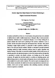
Figure 1: Adaptive scheduling on a rolling time basis. To construct the new problem P1 we remove all tasks oij from P0 with starting times tij < t1 . In doing so we modify the jobs Ji of P0 which cover operations starting in the period from t0 to t1 by decreasing mi and removing the corresponding operations from Ti. If mi = 0 we remove job Ji completely. If a job has been modi ed but not completely removed from the production program we calculate a new release time from the original job Ji by 



ri = 1max t + pi (k) j ti (k) < t1 : km i (k) i

i

i

i

This update procedure is sketched in the two upper charts of Figure 1. The remaining operations of three jobs in P1 appear in light gray shade. Sometimes the processing of a task oij starting shortly before a new job is released overshoots t1 (tij < t1 < tij + pij ). In this situation Mj is not available at the beginning of time t1 , depicted by black shading for M2 and M3. To overcome this situation we calculate new setup times for all machines by 



(t + pij j tij < t1 ) ; t1 : sj = 1max in ij

Finally we add job Jn+1 released at t1 = rn+1 (appears in dark gray shade) to the modi ed production program of P0 and get the new dynamic scheduling problem P1 . After update the production program is rescheduled by the PGA until the next job is released at t2 . Meanwhile all tasks starting before t2 are implemented in the manufacturing system. 4

340 320 mean job flow time

mean job flow time

200 300 280 260 240

100 remaining jobs completed jobs

220 200

0

20

40 60 generations

80

0

100

0

job release times

1000

Figure 2: (left) Adaptation of mean job ow time (F ) for the deterministic test problem reached by PGA. The lower curve shows the performance of PGA using initial seeding (PGA+IS). Figure 3: (right) Temporal decomposition of the same (but nondeterministic) problem. The curves show F calculated by PGA for remaining- and for already completed jobs. We use this decomposition technique to perform adaptive scheduling on a rolling time basis of an evolving sequence of dynamic problems. Whenever a new job is released, we generate a problem in the described manner, then we solve it entirely and nally implement its solution. In this way, the temporal decomposition approach to job shop scheduling opens two important perspectives. First it allows to handle nondeterministic events occurring in manufacturing systems in general, e.g. machine breakdowns. The second aspect refers to a special feature of genetic algorithms. Implementing a problem's solution into the succeeding problem model can also be done for the algorithm itself. Let us consider the nal population of a PGA run. Typically only a small fraction of information in the strings is used to schedule tasks in the last time period. Why not modifying the already adapted strings to the needs of the new problem? Probably it is quite similar to the old problem and the strings can be used as initial population in the run solving the next problem. Up to now we have not tested this idea but it sounds promising.

5 Computational Results The new approaches have been tested on a single 100-jobs/5-machines problem using uniformly distributed release times from the interval [0 ? 1000]. In a rst step we apply PGA with a xed population size and generation number of 100. The upper curve of gure 2 shows the adaptation of mean job ow time for the best so far generated string in terms of generations. In a second experiment (PGA + IS) we parameterize the algorithm identically, but seed the initial population with strings resulting from 100 simulation runs using the RANDOM priority-rule. It can be seen from the lower curve of the gure that initial strings of this run are nearly as good as the best generated strings of our rst approach. Both versions treat the dynamic job shop in total, i.e. they schedule 500 tasks on a whole. This tremendous work causes a relatively weak performance of the randomly initialized version. Notice that it has to force out strings from the population that schedule jobs with late release times early. It is amazing that genuine genetic search nally leads to a solution quality which is approximately reached by a FIFO based simulation. To solve our test problem nondeterministically we decompose into 100 determined job shops arising from the events of job releases (PGA+TD). Each of the 100 runs has to schedule 57 tasks on average and xes about 9% of them in the total schedule. Figure 3 shows the mean ow time for the reduced problems in the upper curve. The expected ow time for the remaining 5

Heuristic F (best) F (mean) sec. MWKR (most work remaining) 352 359.7 13 FIFO ( rst in { rst out) 252 256.5 6 SPT (shortest processing time) 191 196.6 8 PGA (genuine) 236 247.6 145 PGA+IS (initial seeding) 215 218.2 148 PGA+TD (temporal decomposition) 182 187.1 229

Table 2: Simulation results.

(known) tasks decreases if the next event is relatively far away, i.e. PGA can place a lot of starting times in the total schedule. In contrast to blind priority-rules PGA has a restricted view of the future and is therefore able to make decisions on a long term basis, provided enough time is left. The lower curve shows the accumulated mean ow time of already completed jobs. In our three approaches (see Table 2) we implement procedures that consider the entire manufacturing system at each instance of the scheduling problem. In contrast, priority-rules consider only one machine at a time. At least PGA+TD clearly outperforms all other simulation runs, whereas the comparison of the runtimes does not lead to a measure of eciency for adaptive search in dynamic task scheduling.

6 Conclusions In this paper we have outlined how to use genetic algorithms in the domain of dynamic scheduling. Although computational evidence from a single test problem is too small as to serve for de nite conclusions, it might allow us to state a few conjectures. The application of genuine genetic search in dynamic as well as in static scheduling performs poorly for large test problems. A common but still promising way out comes from hybrid population based search by problem speci c heuristics or more general hill climbing methods. For dynamic scheduling temporal decomposition opens a way towards treating real world applications [6]. Temporal decomposition can give us some insight into the levels of solution quality reached by simulation methods. To dominate this level by only a few percent is already a nice perspective. Nevertheless, the exploration of the gap between the best solutions of a production scheduling problem and results coming from simulation still suggests the use of globally acting search techniques.

References [1] Bierwirth, C.: A Generalized Permutation Approach to Job Shop Scheduling with Genetic Algorithms. Special issue on Local Search, OR Spektrum (to appear 1995) [2] Blazewicz, J., Ecker, K., Schmidt, G., Weglarz, J.: Scheduling in Computer and Manufacturing Systems. Springer Verlag, Heidelberg (1993) [3] Gier, B., Thompson, G. L.: Algorithms for Solving Production Scheduling Problems. Operations Research 8 (1960) 487{503 [4] Mattfeld, D.C., Kopfer, H., Bierwirth, C.: Control of Parallel Population Dynamics by Social-Like Behavior of GA-Individuals. In: Davidor, Y., Schwefel, H.-P., Manner, R. (eds): Proc. of PPSN-3, Lecture Notes in Computer Science 866 (1994) 16-25 [5] Raman, N., Talbot, F.: Real Time Scheduling of an Automated Manufacturing Center. European Journal of Operations Research 40 (1989) 222-242 [6] Rixen, I., Bierwirth, C., Kopfer, H.: A Case Study of Operational Just-in-Time Scheduling using Genetic Algorithm. In: Biethahn, J., Nissen, V. (eds) Evolutionary Algorithms in Management Applications, Springer Verlag (to appear 1995) [7] Pesch, E.: Learning in Automated Manufacturing. Physica Verlag, Heidelberg (1994) [8] Van Dyke Parunak, H.: Characterizing the Manufacturing Scheduling Problem. Journal of Manufacturing Systems 10 (1992) 241-259

6