a camera calibration technique using targets of circular features

A CAMERA CALIBRATION TECHNIQUE USING TARGETS OF CIRCULAR FEATURES Ginés García Mateos Dept. Lenguajes y Sistemas Informáticos Universidad de Murcia 30.071 Campus de Espinardo, Murcia, Spain. Mail: [email protected]

Abstract Accurate camera calibration is essential in many computer vision applications, where quantitative information is extracted from the images. This paper deals with the problems of subpixel feature location on the calibration target and its automatic matching with the corresponding 3-D world points, as the first part of an unsupervised calibration process. In the proposed method a grid of circular features is used as target. Feature detection and location is carried out using a very simple and efficient connected component labeling algorithm, which incrementally calculates an ellipsoidal description of the regions. This description is a robust and accurate model of the projected circular features, since the perspective projection of a circle is always an ellipse. Some heuristics are presented for selecting those regions corresponding to circles in the target. From these ellipses, feature points are extracted, considering the effect of perspective. Experimental results have shown high robustness of the method against random noise and defocusing. Subpixel accuracy is achieved and computational complexity is linear with the number of pixels.

1. INTRODUCTION AND PREVIOUS WORK Generically, calibration is the problem of estimating values for the unknown parameters in a sensor model, in order to determine the exact mapping between sensor input and output. There exists a wide range of computer vision applications, such as 3-D reconstruction [6] or stereo [9], that requires an accurate calibration of the visual system. In these applications, certain quantitative information is extracted from the images, and overall performance depends on calibration accuracy. Although there also exists techniques inferring 3-D information from uncalibrated cameras, the counterpart is usually a scale factor indetermination [10]. In the computer vision context, camera calibration is the process of determining the internal physical camera parameters (intrinsic parameters) and/or the 3-D position and orientation of the camera relative to the world reference frame (extrinsic parameters) [1]. A visual system may include one or more cameras and other sensors [6], which should be consistently calibrated. According to [2], four are the main problems when designing a whole calibration procedure: control point location in the images, camera model fitting, image

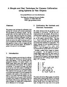
correction for radial and tangential distortion and estimating the errors originated in these stages. While many research has been devoted to model fitting, and some implementations are publicly available [3], few works can be found in the literature about the other stages of the process. This paper addresses the first problem, that of accurately locating feature points in the images. Here, we are free to choose both the design of the calibration target and the detection/location algorithm. In the standard solution described in [10], the target is composed of two planar grids of dark rectangles on a white background. The algorithm locates rectangle corners using a Canny edge detector followed by a Hough transform and line intersections. In [1] Roger Tsai uses contour following in a binarized image for detecting corners in a pattern of rectangles. Wilburn [3] also uses a pattern of rectangular features, shown in Figure 1a), and corner detection but applied on edge images and refined in various steps. Heikkilä and Silvén [2] consider targets of circular features, similar to the one in Figure 2d). They locate feature centroids, correcting perspective effect iteratively. Some other methods are described in [5] using patterns of small dot features, like laser spots. Figures 1b) and 1c) show two other typical targets used in inverse perspective mapping techniques and radial distortion calculation. In both cases only a partial parameter calculation is required.

a)

b)

c)

Figure 1: Some typical targets for camera calibration. The method presented in this paper proposes the use of calibration targets composed of circular features. Contrary to the technique of [2], perspective effect, causing error in feature location, is corrected explicitly in a simple direct form. This allows the grid of features to be of a reduced size, requiring a small grid in each plane. Interest is taken in designing an automatic technique for feature location, so the main objectives are accuracy, robustness and efficiency. The structure of the paper is as follows. Section 2 introduces and justifies the use of targets of circular features. Next, the algorithm for unsupervised detection and location of target features is described. Section 4 deals with the problem of matching image points and 3-D world points. Experimental results, testing accuracy, robustness and efficiency of the method, are reported in section 5. Finally, section 6 briefly discuss the results and accomplishment of the objectives.

2. CALIBRATION TARGETS OF CIRCULAR FEATURES A typical camera calibration target, like those in Figure 1, consists of a grid of uniformly spaced simple features, located in one or more planes, with colours causing a high contrast between the features and the background. The technique proposed in this paper uses circles as the basic component of the target. In fact, elliptical features should also be considered as the problem statement remains the same. Only for construction simplicity circles seem to be more adequate.

a)

b)

c)

d)

Figure 2: Examples of calibration targets of circular features. a) Simple 2-D. b) Simple 3-D. c) Multiple 2-D. d) Multiple 3-D. Figure 2 shows some calibration targets used in the experiments described in section 5. This figure is not a classification but a sample of the variety of possible instances. For example, the arrangement of elements is not necessarily a square grid. 2-D targets only allow a partial recovery of calibration parameters. In this context, a target is called simple when feature grid size is the minimum possible being regular, namely a 2x2 grid of circles. Targets of circular features have already been used in several camera calibration works, like [2, 5] and references therein. The key idea to justify the use of circles is the fact that perspective projection of a circle, or in general of an ellipse, is always a circle or an ellipse. A simple graphical proof appears in Figure 3, a formal demonstration can be found in [2]. The rays coming from the camera focus C and going throw the circle RW form a skewed cone in the world space. Perspective projection of RW, labelled RIM, can be obtained as the intersection of image plane P and this skewed cone, so RIM boundary is defined by a quadratic curve. In practice, RIM will always be a circle or ellipse. Now, suppose we are designing an algorithm for locating features in the target. The centroid of the projected circles could be located easy and accurately. However, it's well known that e', the projected centre e of circle RW, is not necessarily mapped to the centroid of RIM. In fact, e' cannot be located without using any additional information, as there exists a many to one mapping between all possible RW and RIM. This perspective effect on circular features has made many researchers to avoid using circles in calibration targets. Some solutions have been designed to try to correct this effect, by iteratively correcting feature locations [2] or minimising perspective bias using dots as target features [5]. Section 4 proposes a more direct

solution to the problem: invariant features can be located on the projected circles considering the relations among coplanar circles.

o

C

e'

e

o

RIM

Rw P

Figure 3: Perspective projection of a circle is always an ellipse, but ellipse centroid is not necessarily the projected centroid of the circle. The previous justification of circular features supposes that perspective projection, or equivalently a pinhole camera model, is used. When radial and tangential distortion are considered circles may not be mapped to ellipses. This effect is more evident for high distortion values and is not easy to model. Section 4 presents two ideas to overcome this problem. 3. AUTOMATIC FEATURE DETECTION AND LOCATION In the camera calibration field, techniques for feature detection and location are primarily concerned with accurate subpixel location of the measured features. When the calibration procedure is integrated in an automatic system, process execution becomes unsupervised, allowing the system to recalibrate itself when adequate conditions are found. Therefore, two other criteria have to be considered: efficiency in terms of execution time and robustness with non ideal images. In order to meet these objectives of accuracy, efficiency and robustness, the proposed method keeps the processing level as low as possible. Not highly elaborated feature descriptors are used, in contrast with the use of edge and line information. Specifically, gaussian descriptors for blobs of connected pixels are calculated. Following subsections describe the designed method in detail. 3.1. The Process for Automatic Calibration The process for automatic calibration proposed in this paper is presented in Figure 4. The underlying structure consists of three sequential stages: detection of circular features, matching image points with 3-D world points and model fitting to calculate calibration parameters. Image correction and error estimation stages are not considered here as a part of automatic calibration.

ACQUISITION

TARGET DESCRIPTION

Target images BINARIZATION

3-D world points Circle positions

REGION GROUPING POINT MATCHING

Point pairs image/world

DESCRIPTION

Image points

Region list SELECTION OF TARGET COMPONENTS

Ellipse list

ELLIPSE MATCHING AND FEATURE POINT CALCULATION

CAMERA MODEL FITTING

Calibration parameters CALIBRATED SYSTEM

Figure 4: Automatic calibration process using circular features. Input: acquisition and target description. Output: calibration parameters. Firstly, circles in the target are individually detected and located, which implies three tasks: image binarization, connected component grouping and description of these components. In fact, they all can be accomplished simultaneously, by adequately defining the main step of a connected component labelling algorithm, thus requiring a single scan of the image. Next, an heuristic step is applied to reject spurious regions resulting from noise or background objects. Since the grid structure of features is known a priori, the matching of detected ellipses with circles on the target can be made with a topographic sorting of the regions. This matching is required by the feature point calculation, described in section 4. Resulting points can be directly matched with the corresponding world points of the target. Finally, a camera model fitting technique is applied. As mentioned above, this paper is not mainly concerned with this part of the problem. Some solutions have been proposed. They all take as input pairs of image and world points, and solve for the parameters of the model. In some of the experiments, direct linear transformation (DLT) method [9] was used, although results are not discussed here. 3.2. Algorithm for Ellipse Detection and Location The process of detection and accurate location of the features in the pattern is essentially a connected component labelling algorithm, like the one explained in [11]. This algorithm makes an ordered scan of all the pixels in an image, from left to right and from top to bottom. For each pixel, its processed neighbours are considered and then an adequate action is taken: adding the pixel to a component, creating a new component or joining two existing components. 4-connectivity is

used here. Defining appropriate additional actions, the tasks of binarization and region description can be made during the same scan. For the binarization, the algorithm should only consider pixels under a certain threshold, no explicit binarization is required. Thresholding can be fixed or adaptive, the better solution is application dependent. Calibration target characteristics enable to use a relatively simple solution: a partial histogram (that is, considering only some of the pixels) of grey levels is calculated and then the threshold is located approximately in the median value. For the component description, bidimensional gaussian descriptors are used, containing five parameters for each component E = ( x , y , σx2, σy2, σxy). Suppose region E is assigned the set of pixels PE = {(xi, yi), i= 1..n}. Gaussian parameters are easily computed accumulating the sums of xi, yi, xi2, yi2 and xi·yi, and applying the following formulas:   (x, y) = ∑ x i / n, ∑ yi / n  (1)   i =1..n i =1..n 2 2   (σ 2x , σ 2y , σ xy ) =  ∑ x 2i / n − x , ∑ y2i / n − y , ∑ x i yi / n − x y  (2) i =1..n   i =1..n i =1..n So component description is made by adding a reduced number of computations in each step of the algorithm, and a final computation at the end. The algorithm described in [11] requires a double scanning of images, because when two components are joined all their members have different labels. This can be avoided using an equivalence table of components [12], so pixels aren't assigned labels but indices in the table. In this implementation, components are stored in an equivalence tree structure, and operations on the table use two techniques known as path compression and weighted union. Operations on this structure are of nearly constant cost, so total cost of the process is linear with the number of pixels. 3.3. Selection of Elliptical Components of the Target While gaussian descriptors are used in many computer vision applications as coarse shape approximations, here gaussians are the more accurate and adequate possible election. The reason was given in section 2: perspective projection of a circle is always an ellipse. In fact, gaussians are not only accurate but robust descriptors obtained by accumulation of the contributions of all shape interior pixels. Ellipse parameters can be obtained from the gaussian parameters µ = ( x , y ) and Σ = ((σx2, σxy), (σy2, σxy)) using the following formulas: - Ellipse centroid: µ. - Ellipse mayor and minor axes: first and second eigenvectors of Σ. -

Ellipse mayor and minor radius: 2 σ 2v1 and 2 σ2v2 , being σv12 and σv22 the first and second eigenvalues of Σ, respectively.

But other components may also correspond to non elliptic shapes, caused by objects in the background of the scene. This is particularly important when automatic unsupervised calibration is considered. A simple test can be applied for selecting elliptic shape components. Suppose we have an ellipse R. Its area SR is a function of its mayor and minor radius, a and b, according to SR = πab. Applying the relations above, we have that the expected number of pixels for an elliptical component is: Pixel count (R ) ≈ S R = 4π σ 2v1 ⋅ σ 2v 2 = 4π σ2x ⋅ σ 2y − (σ xy )2

(3)

This property only holds for ellipses, so it is a simple test for rejecting non elliptical components. Other heuristic criteria can be used to remove spurious components, not corresponding to circular features, like the size of the component or its distance to other components. 4. LOCATING AND MATCHING FEATURE POINTS The list of ellipses resulting from detection, location and selection is a robust and accurate description of the circular features of the target in input images. However, camera model fitting techniques for parameter calculation require as input a set of corresponding points, in image and world coordinates, so extraction of feature points is needed. In the case of circular features, the problems of correspondence and feature point location are closely related. As mentioned above, no invariant feature point can be extracted from a single isolated ellipse resulting from a projected circle. But invariant feature points can be obtained when relations between coplanar ellipses are considered. Thus, ellipse correspondence problem is prior to point location and point correspondence is made after point location. In short, first ellipses in the images are matched with circles in the target. Then feature points are calculated for each of the ellipses, and finally those points are associated with corresponding 3-D world points. This last correspondence step is trivial, as matching of circular features is known. On the other hand, although matching of image ellipses with target circles is not a trivial task, it's neither a complex one. In the experiments, it has been observed that after region selection, described in subsection 3.3, nearly all resulting ellipses do certainly correspond to circular features in the target. Usually, existing background objects in the scene are rejected or result in small size elliptic shapes, so they can also be easily removed. Therefore, matching can be accomplished with a simple topographic sorting of the ellipses (for example, top to bottom and left to right, using adequate angles for the sort criterion) associating them with target features in the same order. Some heuristic criteria of size or distance could be used for removing possible remaining spurious ellipses.

4.1. Feature Points in a Target of Circular Features A family of interesting invariant feature points results from tangent lines that are common to two coplanar circumferences. For every two coplanar circumferences with a null intersection, there exist exactly four common tangent lines. Suppose a line R, which is tangent to circumferences C1 and C2, located in the same plane of a calibration target, as shown in Figure 5a). After perspective projection, see Figure 5b), the projection of R, labelled as R', is a common tangent of E1 and E2, projection of C1 and C2, respectively. Consequently, the property of being a common tangent to two coplanar circumferences remains invariant to perspective projection. In general, this property holds for any shape. So, for this problem, intersection points of these common tangents and the ellipses can be used as accurate and easily calculable feature points. E1

C1 p1

q' 1

p' 1

q1 R

R'

q' 2

q2 p2 C2

a)

p' 2

E2

b)

c)

Figure 5: Feature points in a target of circles. a) Two coplanar circumferences and their common tangents. b) A perspective projection of a): common tangent property remains invariant. c) Possible feature points calculated using common tangents. A common tangent to two ellipses may leave both in the same side, as R' in Figure 5b), or may leave each one in a different side, as the line going through q'1. For an arrangement in square grid of circles, calculating intersection points in world coordinates is trivial using tangents of the first type. For example, in the grid of Figure 5c), with circles of radius r, for each circle in XY plane, centered in (x, y, z), its four feature points are (x±r, y, z) and (x, y±r, z). These are drawn as grey dots. Other feature points can be calculated using common ellipse tangents. Making appropriate intersections of tangent lines, feature points marked with X in Figure 5c) are obtained. Projected centers of circular features are also calculated intersecting two lines: the one going through points associated to (x±r, y, z) and the one going through points associated to (x, y±r, z). The underlying geometrical problem is to calculate the four common tangent lines to any two ellipses. Although it has been proven that a closed form solution exists for this problem, the formulae are so large that another method is preferable (the formula for a simplified version, obtained with a computer program, fills more

than 5 pages of plain text). An alternative is to make an iterative calculation, solving many times the problem of calculating the tangent to an ellipse going through a given point. This process works as follows. We start fixing a point p1 in an ellipse E1 and calculate points p2 and p'2 of the tangents in the other ellipse E2 (the tangents to E2 going through p1). Now p2 and p'2 are fixed and tangent points are calculated in E1 (four points result, so adequate solutions are to be selected) and set p1 and p'1. Then p2 and p'2 are recalculated and so on. It can be proven that this process converges. Experimentally, convergence is very fast and usually less than one iteration is required for each decimal digit of accuracy. 4.2. Dealing with Radial and Tangential Distortion So far, it has been considered that radial and tangential distortion effects are negligible. Some conclusions may not hold when they are taken into account: circles are not mapped to ellipses and tangent invariance may not always be true, because lines are not necessarily mapped to lines. However, the proposed technique is a good approximation for typical distortion values. A possible technique for explicitly dealing with distortion is to make an iterative process, where calibration parameters are refined in each step until convergence is reached. First, feature point location is applied to the original distorted image and then a model fitting algorithm calculates the camera parameters. Using these initial parameter values, image is corrected for radial and tangential distortion and next, feature point location is applied to it. Using these new image points, parameters are recalculated, obtaining closer approximations to the real values. The process is repeated until desired accuracy is obtained. This iterative structure, of point and parameter recalculations, is similar to the solution proposed in [2] to compensate perspective effect in circular features. Convergence is expected to be reached in a few iterations. In the experiments, described in the following section, another solution has been used. First, radial and tangential distortions have been estimated. Then, images are corrected for distortion and the remaining parameter can be calculated in an accurate way. This is a simpler solution, but the problem here is how to make the first step. An approximate solution has been used, with a partial calibration applied to the result of feature location in distorted images. This is equivalent to apply two iterations of the method described above. 5. EXPERIMENTAL RESULTS Some tests have been carried out to measure the quality of the proposed technique. The main interest of experimentation is the process for feature detection and location described in this paper. Thus, the objective of tests is three-fold: accuracy in feature point location, robustness to noise and defocusing and efficiency. A low cost off-the-self acquisition system is used (a QuickCam Pro vide-

oconference camera). Image resolution is 320x240 at 256 grey levels. For the results described here, calibration target of Figure 2a) was used. Some experiments with the other targets showed similar results. Images are a priori corrected for distortion, as explained in subsection 4.2, and feature points are projected centers of the circles. Usually, feature location accuracy is measured after calibration parameters are obtained, which supposes that these parameters are the real values. Here another method is applied, comparing resulting locations with a manual measure. This measure is made by manually selecting auxiliary lines in Figure 2a) in 300% scaled images, so its estimated accuracy is not better than 1 / 3 2 pixels. Location accuracy tests are shown in Figure 6a). Mean accuracy in point location is measured for different sizes of ellipses in the images (a total of 30 samples were used), varying target distance and viewing angle. Bars indicate minimum and maximum point error. Mean error of 0.43 pixels is nearly independent of ellipse size and observed oscillations are not significant. Standard deviation is 0.19 pixels, and the target was detected in 97% of the samples. a) Location error vs. ellipse size in images 1.0

Manual measure accuracy

0.8 0.6 0.4 0.2 0 10

15

20

b) Execution time vs. image size

Execution time (ms.)

Location error (pixels)

1.2

25

30

35

140 120 100 80 60 40 20 0

160

Mean ellipse radius (pixels) c) Location error vs. gaussian sm o o thing

480

640

800

d) Location error vs. random noise

1. 4 Location error (pixels)

1.2 1.0 0.8 0.6 0.4 0.2 0 2 3 4 5 6 1 Gaussian sm o o thing level, σ

320

Image width (pixels)

7

0.8 0.6 0.4 0.2 0 0%

10%

20%

30%

40%

Noise percentage (in each pixel)

Figure 6: Results of the test of location accuracy a), computational efficiency b), robustness to gaussian smoothing c) and random noise d). Subpixel accuracy is clearly reached, but the value is so close to error introduced by the manual measure that another method is needed for an appropriate accuracy estimation. Synthetic samples of the target have been generated, with approximately the same locations of feature points in real samples. For these synthetic samples, ground-true positions are exactly known, so error measures are more reliable. In this case, accuracy was 0.05 pixels with a standard deviation of 0.03 and maximum error

of 0.13 pixels. This is an order of magnitude better than other techniques using square features, like [1] that reports 1/2 to 1/3 pixel accuracy, of [3] with 0.335 mean pixel error in the best case. In [2] circular feature detection accuracy is about 0.02 pixels, but they use a grid of 40x40 circles, so efficiency and robustness are difficult to be accomplished. Something similar happens when comparing with spot feature techniques [5], that reach accuracy values of less than 0.01 pixels. Efficiency tests showed that computational complexity is linear with the number of points. Times shown in Figure 6b) have been measured in a K6 at 350 Mhz. including only feature detection and location The whole process, considering input/output and parameter calculation, can be made in real time in a PC, at a frequency of about 10 Hz. As far as robustness is concerned, two kinds of distortions have been considered: gaussian smoothing and random noise, applied to some of the real images, so ground-true values are that of manual calibration. Although error slowly increases with defocusing, the subpixel accuracy is maintained even for very high distortion values. More importantly, calibration target remains detected under these extreme circumstances. No similar tests have been found in the literature for comparison with other methods. 6. CONCLUSIONS For a calibration technique to be executed in an unsupervised framework, the process should meet certain criteria of accuracy in the obtained parameters, computational efficiency and robustness with noisy images. This paper deals with the first stage of a calibration process, that is, locating feature points in a target, whose world coordinates are known. The key idea of the proposed method is to use calibration targets composed of circular features and compensate perspective effect by calculating invariant points, resulting from common tangents to coplanar ellipses. Circular feature detection and location becomes a simple connected component labelling process in a binarized image. Each component is described by its mean and covariance matrix. This gaussian description is highly accurate and robust, as projection of circles are circles or ellipses. Then, ellipses are matched with circular features in the target and finally feature points are obtained using geometrical calculations. Experimental results show that the proposed method meets all the desired objectives. Subpixel accuracy is obtained in the location of feature points. The real accuracy of the method (that is, not considering the error due to manual calibration) is in the order of 0.05 pixels. This is better than many existing methods and comparable to the more accurate ones. But subpixel accuracy is not only reached for ideal images, but is maintained for highly corrupted images, considering gaussian defocusing and random noise. These conditions are not applicable to many existing methods, limiting their use in automated contexts. As far as computational efficiency is considered, the algorithm is linear with the number of pixels, requiring a single scanning of the image.

7. ACKNOWLEDGEMENTS Thanks to P.E. Lopez-de-Teruel, Cristina Vicente and Alberto Ruiz, for the revision of this paper. This work has been supported by CICYT project TIC98-0559. References [1] R.Y. Tsai, “A Versatile Camera Calibration Technique for High-Accuracy 3-D Machine Vision Metrology Using Off-the-Shelf TV Cameras and Lenses”, IEEE Journal of Robotics and Automation, vol. ra-3, no. 4, 1987. [2] J. Heikkilä and O. Silven, “A Four-step Camera Calibration Procedure with Implicit Image Correction” in Proceedings of the 1997 IEEE Conference on Computer Vision and Pattern Recognition, June 1997, pp. 1106-1112. [3] B. Wilburn, “Automatic Feature Point Extraction for Light Field Camera Calibration”, Project Report, in Stanford University, Electrical Engineering Dept., http://velox.stanford.edu/~wilburn/Calibration/report.html. [4] C. Chatterjee and V. Rowchowdhury, “Efficient and Robust Methods of Accurate Camera Calibration”, IEEE Computer Vision and Pattern Recognition, pp. 664-665, 1993. [5] T.A. Clarke, “An analysis of the properties of targets used in digital close range photogrammetric measurement”, Videometrics III, SPIE vol. 2350, pp. 251- 262, Boston, 1994. [6] J. C. Sabel, Calibration and 3D Reconstruction for Multicamera Marker Based Motion Measurement, Delft University Press, 1999. [7] G.Q. Wei and S.D. Ma, “Implicit and Explicit Camera Calibration - Theory and Experiments”, IEEE Transactions on Pattern Analysis and Machine Intelligence, 16(5), pp. 469-480, 1994. [8] S.K. Kopparapu and P. Corke, “The Effect of Measurement Noise on Camera Calibration Matrix”, IVCNZ 98, Auckland, New Zealand, 1998. [9] O.D. Faugeras and G. Toscani, “Camera Calibration for 3D Computer Vision”, in Proc. of Intl. Workshop on Industrial Applications of Machine Vision and Machine Intelligence, Silken, Japan, pp. 240-247, 1987. [10] E. Trucco and A. Verri, Introductory Techniques for 3-D Computer Vision, Prentice-Hall, 1998, pp. 123-138. [11] R.C. González and R.E. Woods, Digital Image Processing, AddisonWesley, 1992, pp. 40-71. [12] A.V. Aho, J.E. Hopcroft and J.D. Ullman, Data Structures and Algorithms, Addison-Wesley, 1983.