J. Europ. Opt. Soc. Rap. Public. 9, 14044 (2014)
www.jeos.org
Improving the Generic Camera Calibration technique by an extended model of calibration display T. Reh
¨ angewandte Strahltechnik, Klagenfurter Str. 2, 28359 Bremen, Germany BIAS - Bremer Institut fur
[email protected]
W. Li
VEW - Vereinigte Elektronik Werkst¨atten GmbH, Edisonstr. 19, 28357 Bremen, Germany
J. Burke
¨ angewandte Strahltechnik, Klagenfurter Str. 2, 28359 Bremen, Germany BIAS - Bremer Institut fur
R. B. Bergmann
¨ angewandte Strahltechnik, Klagenfurter Str. 2, 28359 Bremen, Germany BIAS - Bremer Institut fur University of Bremen, Faculty of Physics and Electrical Engineering, Applied Optics, Otto-HahnAllee 1, 28359 Bremen, Germany
Generic camera calibration is a method to characterize vision sensors by describing a line of sight for every single pixel. This procedure frees the calibration process from the restriction to pinhole-like optics that arises in the common photogrammetric camera models. Generic camera calibration also enables the calibration of high-frequency distortions, which is beneficial for high-precision measurement systems. The calibration process is as follows: To collect sufficient data for calculating a line of sight for each pixel, active grids are used as calibration reference rather than static markers such as corners of chessboard patterns. A common implementation of active grids are sinusoidal fringes presented on a flat TFT display. So far, the displays have always been treated as ideally flat. In this work we propose new and more sophisticated models to account for additional properties of the active grid display: The refraction of light in the glass cover is taken into account as well as a possible deviation of the top surface from absolute flatness. To examine the effectiveness of the new models, an example fringe projection measurement system is characterized with the resulting calibration methods and with the original generic camera calibration. Evaluating measurements using the different calibration methods shows that the extended display model substantially improves the uncertainty of the measurement system. [DOI: http://dx.doi.org/10.2971/jeos.2014.14044] Keywords: Camera calibration, generic camera calibration, active grids, fringe projection, 3D metrology
1 INTRODUCTION Todays camera calibration methods are almost exclusively based on the pinhole model, usually extended with a simple distortion function [1]–[4]. In contrast to these photogrammetric models that typically contain very few parameters, Grossberg and Nayar [5] proposed a model-free approach, in which every pixel is characterized by the half-ray in space from which it collects incoming light. Sturm and Ramalingam developed the method further to work with unknown viewing positions of the calibration objects [6, 7]. This generic camera calibration has already gained some attention for being able to characterize cameras with fisheye or catadioptic lenses with a field of view larger than 180◦ [8]. These systems cannot be described by a projection onto an image plane (even with strong distortions) or simply do not have a single centre of projection. Because the approach of generic camera calibration is modelfree, the half-rays of the pixels can be described in every one of these cases. Generic camera calibration can also offer advantages when used in systems with lenses that have very little pincushion or barrel distortion and thus seem to be ideal candidates for the traditional pinhole-based calibration approaches. Bothe et al. [9] have shown that optical metrology systems can achieve
higher accuracy when characterized with generic camera calibration in comparison to traditional photogrammetric calibration. This is due to the fact that the distortion functions only model variations that occur across the whole image. High frequency distortions and other deviations from specific distortion models cannot be described by them, but are automatically included in the single-pixel-based rays of generic camera calibration. The state of the art procedure for generic camera calibration [8, 9] is as follows: Image data of a reference object is captured in a multitude of positions. This object is a monitor displaying active patterns. With a numerical optimization procedure the half-rays of all pixels are then computed from this data (see Section 2). In this article we propose a way to further optimize the use of generic camera calibration in high-performance metrology systems. We show that at this level of accuracy it is necessary to take several issues of the calibration object into account: The used generators of active patterns are neither ideally flat nor do they have zero extent in the direction of the surface normal. We present additional models for the calibration refer-
Received July 31, 2014; revised ms. received September 23, 2014; published October 04, 2014
ISSN 1990-2573
J. Europ. Opt. Soc. Rap. Public. 9, 14044 (2014)
T. Reh, et al.
ence and show that they are appropriate to further enhance the accuracy of the calibration.
2 CALIBRATION WITH ACTIVE GRIDS Traditional photogrammetric camera calibration usually uses flat patterns as reference objects: certain features (e.g. corners of a chessboard pattern) are located on several captured images of the patterns and these coordinates are then used to calculate the model parameters of the camera [4]. However these features are sparse in the image (typically in the range of 102 features for 106 pixels). To apply the generic camera calibration idea of describing a separate ray for each pixel, the data would have to be interpolated. This is what Sturm and Ramalingam did in their first approach to generic camera calibration [7].
𝛼
𝑛 𝑑
ℎ 𝛽
𝛼
𝐱𝐱
𝐱
𝑔 ∆glass
FIG. 1 Refraction of light at the glass cover of the display with thickness d and refractive index n. The illuminated point x appears in the position x’ when viewed under the
Dunne et al. [8] and Li et al. [10] independently developed another method of collecting the calibration data. Instead of static patterns they used active grids presented on a flat screen. By using phase-shifted sinusoidal fringes [11], this approach makes it possible to measure a correspondence for every single pixel of the imaging device. As with static patterns, these correspondences are from an image coordinate (pixel) to a point in the local coordinate system of the calibration object. To fit a line of sight, we need to know several of these points in a common global coordinate system. Therefore it is necessary to know the measurement poses of the display. Usually the end results of the poses are computed by using bundle adjustment, which builds on numerical optimization methods such as the Levenberg-Marquardt algorithm [8]. These methods always need a starting point, from which the optimization then finds a local minimum. There are several methods for finding these initial poses. The method proposed by Sturm and Ramalingam [7] relies on the trifocal calibration tensor and covers the most general case of an image sensor, which leads to considerable mathematical complexity. Dunne et al. [8] developed the synthetic image plane which is particularly useful when calibrating image systems that do not adhere to a pinhole model but still have a single centre of projection. However the cameras and lenses used in the experimental work described below are very pinhole-like and therefore we do not need to use these special methods. Instead the traditional photogrammetric camera calibration [1] can be used to find the initial poses.
angle α. See text for how an expression for the shift ∆glass is derived (using the helper variables g, h, β).
We now present two extensions of this model. First, we allow for deviation from the ideal of a flat plane. This can be modelled by adding a component in normal direction of the plane. Because the deviation is expected to vary only slowly, the component is modelled as a bivariate polynomial ∆plane (u, v) =
The simplest way of describing the display is to assume that the measured (sub-)pixel values lie on a flat surface. Without loss of generality the object coordinate system of the display can be laid out with the xy-plane in this surface and the origin at the top left corner of the display. Thus the corresponding object coordinates for an active grid measurement of (u, v) are
pu x0 (u, v) = pv , 0 with p being the pixel pitch of the display.
(1)
aij ( pu)i ( pv) j ez ,
(2)
2≤ i + j ≤ n
where aij are the coefficients and ez is the unit vector in zdirection. The constant and the 1st order term are omitted on purpose because they are equivalent to a coordinate shift and a scaled rotation respectively. The other extension we introduce concerns the glass cover which is protecting the active part of the display. Due to refraction in this layer, the measured pixels appear in slightly shifted position, which varies with the angle of incidence. Figure 1 shows how the original display point x appears in the shifted position x’. From Figure 1 follows h = d tan β = g tan α,
(3)
which can be rewritten as g=d
3 DISPLAY MODEL
∑
tan β cos α . =d q tan α n 1 − sin2 β
(4)
With d = g + ∆glass and Snell’s law sin α = n sin β this results in ! cos α ∆glass (u, v) = d 1 − p ez (5) n2 − sin2 α where the expression has been vectorized with the unit surface normal ez .
4 EXPERIMENTS An example fringe projection system consisting of two cameras and one projector was constructed to test the effects of
14044- 2
J. Europ. Opt. Soc. Rap. Public. 9, 14044 (2014)
A
glass covered B
10 µm
uncovered
B
D
5 mm
𝑝𝑝99% = 10.4 µm
FIG. 2 Experimental setups. (a) The fringe projection systems with two cameras and one projector with a planarity standard (see text). (b) Calibration setup with 0.77”
𝑝𝑝99% = 21.1 µm
𝑝𝑝99% = 7.0 µm
-10
polynomial
C
𝑝𝑝99% = 15.8 µm
0
flat
A
T. Reh, et al.
micro-OLED display as active grid; The pictured fringe periods are in both cases larger
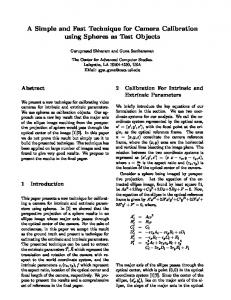
FIG. 3 Result of a measurement of the planarity standard with the fringe projection
than during the actual experiments so as to be visible in the figure.
system. Plots show the deviation of the data from their respective best-fit plane. Identical raw data were processed with calibrations based on the four different display
the extended generic calibration. The cameras both consisted of a monochrome CCD (Manta G-145B, Allied Vision Technologies GmbH, Stadtroda, Germany) and a 25 mm fixed focal length lens (LM25JC10M, Kowa Co. Ltd., Nagoya, Japan). The fringe projection system is pictured in Figure 2(a). For displaying the active calibration patterns during calibration a monochrome green 1280×1024 pixel 0.77” micro-OLED display (SXGA OLED-XLTM , eMagin Corporation, Hopewell Junction, USA) was used. According to manufacturer specification, the pixel pitch of the display is 12 µm and the glass cover has a thickness of 0.7 mm, with a refractive index of 1.52 for green light. Calibration data were collected for both cameras inside the focused volume in a separate calibration setup (see Figure 2(b)). In total the display was measured in 45 different positions for each camera. The fringe projection system was then used to measure a planarity standard. To be measurable for the system, the standard must have a high amount of diffuse reflection, i.e. it must have a high roughness. On the other hand the roughness has to be small enough to not interfere with the planarity of the standard. The best commercially available compromise was a ceramic of size 50×50 mm2 with a known maximum planarity deviation of 2.7 µm (AiMESS Products GmbH, Burg, Germany).
5 EVALUATION The calibration data were used to perform four different calibrations of the fringe projection system with the following models for the active grid display: A. flat surface (x = x0 ) B. flat surface covered by glass (x = x0 + ∆glass ) C. polynomial surface (x = x0 + ∆plane ) D. polynomial surface covered by glass (x = x0 + ∆glass + ∆plane )
models (see Section 5): A) flat display surface; B) flat display surface covered by glass; C) polynomial display surface; D) polynomial display surface covered by glass; The denoted quantity is peak-to valley of 99% of the data. It can be seen that model D produces the best results among all tested methods.
For the glass cover thickness and refractive index we used the values specified by the manufacturer. The polynomial coefficients were initialized with zero and then varied as additional parameters in the bundle adjustment. This yields four different calibration results, one for each of the display models. Each of these four calibration results was used to evaluate the measurement data of the planarity standard. So for each single measurement of this standard, we obtained four different results, one for each of the display models.
6 RESULTS AND DISCUSSION To judge the quality of the different results, a plane was fitted through each of the measurement results and the distance of the data points to this plane was computed. These deviations are plotted for one of the measurements in Figure 3. The most noticeable improvement is clearly the inclusion of the polynomial plane surface (C). On the other hand the glass cover model alone (B) decreases the quality, but the combination of both display model extensions (D) yields the best result among all tested models. It can be seen that the measurement result with the flat display (A) is curved considerably, while the polynomial plane display model (C) reduces this significantly. This suggests that the used reference display is not flat. By assuming it is flat, a certain “warp” is incorporated into the calibration A. Thus, the measurement results of the planarity standard contain the curvature seen. The finding of a less warped measurement result when using display model C suggests that this calibration automatically allows the bivariate polynomial to converge to the real surface shape of the display. Therefore the calibra-
14044- 3
J. Europ. Opt. Soc. Rap. Public. 9, 14044 (2014)
T. Reh, et al.
tion C does not incorporate the warp that has been encountered in A. A possible explanation for the low impact of the glass cover model (B) is that the calibration display of the test system was very small (diagonal 0.77” = 19.6 mm). This means that the angle of incidence α varies very little across the display for each measurement. Therefore ∆glass (Eq. (5)) is basically a constant shift for each measurement frame. For other combinations of optics and calibration display with larger variance of α the impact of the glass cover might be bigger. This is not possible with the current set-up but to be investigated in further work. To evaluate the reduction of the measurement uncertainty, the peak-to-valley reading (after removing 1% as outliers) was taken. The combined models (D) improved this value from 15.8 µm to 7.0 µm and is therefore by far superior to the other models.
7 SUMMARY In this article we presented an approach for improving the generic camera calibration when using active grids as calibration objects. The traditional approach of assuming a completely flat display surface (model A in this paper) is enhanced with two new additions: 1) refraction in the glass that covers the display rendering these grids (B) and 2) deviations of the active grid surface from ideal flatness (C). These two improvements have been tested separately and in combination (D), with experimental data from an example micro fringeprojection system. The results show that the combined models bring about a significant improvement with regard to their separate implementations, as well as the traditional model of a completely flat display. The uncertainty of the fringe projection measurement was reduced by a factor of 2 with method D.
References [1] Z. Zhang, “A flexible new technique for camera calibration,” IEEE Trans. Pattern Anal. Machine Intell. 22, 1330–1334 (2000). [2] P. F. Sturm, and S. J. Maybank, “On plane-based camera calibration: a general algorithm, singularities, applications,” in Proceedings to the IEEE Conference on Computer Vision and Pattern Recognition, 432–437 (IEEE, Fort Collins, 1999). [3] R. Hartley, and A. Zisserman, Multiple view geometry in computer vision (second edition, Cambridge University Press, Cambridge, 2004). [4] G. Bradski, and A. Kaehler, Learning OpenCV (O’Reilly, Sebastopol, 2008). [5] M. Grossberg, and S. Nayar, “A general imaging model and a method for finding its parameters,” Proceedings to the 8th IEEE International Conference on Computer Vision, 108–115 (IEEE, Vancouver, 2001). [6] S. Ramalingam, P. Sturm, and S. K. Lodha, Theory and experiments towards complete generic calibration (INRIA - Institut national de recherche en informatique et en automatique, RR-5562, 2005). [7] P. Sturm, and S. Ramalingam, A generic calibration concept theory and algorithms (INRIA - Institut national de recherche en informatique et en automatique, RR-5058, 2003). [8] A. K. Dunne, J. Mallon, and P. F. Whelan, “Efficient generic calibration method for general cameras with single centre of projection,” Comput. Vis. Image. Und. 114, 220–233 (2010). [9] T. Bothe, W. Li, M. Schulte, C. von Kopylow, R. B. Bergmann, and W. P. O. Jüptner, “Vision ray calibration for the quantitative geometric description,” Appl. Opt. 49, 5851–5860 (2010). [10] W. Li, M. Schulte, T. Bothe, C. von Kopylow, N. Köpp, and W. Jüptner, “Beam based calibration for optical imaging device,” in Proceedings to the 3DTV Conference, 1–4 (IEEE, Kos, 2007). [11] J. Burke, “Phase decoding and reconstruction,” in Optical methods for solid mechanics, P. Rastogi, and E. Hack, eds., 83–139 (WileyVCH, Weinheim, 2012).
8 ACKNOWLEDGEMENTS The work leading to these results has received funding from the European Community’s Seventh Framework Programme under grant agreement no. FP7-285030.
14044- 4