A Capacity Constrained Production-Inventory System with Stochastic

International Journal of Production Research

ee

rP Fo A Capacity Constrained Production-Inventory System with Stochastic Demand and Production Times

Manuscript ID:

Complete List of Authors:

13-Aug-2009

Axsäter, Sven; Lund University, Industrial Management and Logistics INVENTORY MANAGEMENT, PRODUCTION PLANNING

ly

On

Keywords (user):

Original Manuscript

w

Keywords:

TPRS-2009-IJPR-0477.R1

ie

Date Submitted by the Author:

International Journal of Production Research

ev

Manuscript Type:

rR

Journal:

http://mc.manuscriptcentral.com/tprs Email: [email protected]

Page 1 of 12

Fo

A Capacity Constrained Production-Inventory System with Stochastic Demand and Production Times

ee

rP

Sven Axsäter Lund University

iew

ev

rR

ly

On

1 2 3 4 5 6 7 8 9 10 11 12 13 14 15 16 17 18 19 20 21 22 23 24 25 26 27 28 29 30 31 32 33 34 35 36 37 38 39 40 41 42 43 44 45 46 47 48 49 50 51 52 53 54 55 56 57 58 59 60

International Journal of Production Research

Revised August 2009

http://mc.manuscriptcentral.com/tprs Email: [email protected]

International Journal of Production Research

Abstract This paper considers a simple model of a capacity constrained production-inventory system with Poisson demand. The system is controlled by an S policy. The production time for a unit is modeled as a gamma distributed stochastic variable. Using M/G/1 queuing theory it is very easy to evaluate holding and backorder costs and optimize the ordering policy. The suggested model may be useful when evaluating investments in production.

Fo

Keywords: Production-inventory management, Capacity constrained, Stochastic

iew

ev

rR

ee

rP ly

On

1 2 3 4 5 6 7 8 9 10 11 12 13 14 15 16 17 18 19 20 21 22 23 24 25 26 27 28 29 30 31 32 33 34 35 36 37 38 39 40 41 42 43 44 45 46 47 48 49 50 51 52 53 54 55 56 57 58 59 60

http://mc.manuscriptcentral.com/tprs Email: [email protected]

Page 2 of 12

Page 3 of 12

1

1 Introduction In this paper we consider a simple integrated production-inventory system facing Poisson demand. The production capacity is constrained and the production time is stochastic and follows a gamma distribution. Our purpose is to illustrate in a simple way the impact of both capacity limitations and variations in the production times. Our model may be a useful tool when evaluating different capacity investments, which may affect both the mean and the variance of the production time. The impact of capacity investments can, of course, also be evaluated by simulation. However, the

Fo

tool we provide is, in general, much simpler and quicker to use. The planning of capacity investments has been considered in several papers. A recent review of

rP

strategic capacity planning is given by Geng and Jiang (2009). Vits et al. (2007) provide a model to study myopic and long-term process change strategies.

ee

In this paper it is assumed that there are no ordering costs, so there is no need for batch-ordering. The production system can handle only one item at a time. The

rR

system is controlled by a so-called S policy. When the inventory position (stock on hand plus outstanding orders and minus backorders) has reached S no more orders are

ev

triggered until a new demand occurs. By outstanding orders we mean orders that have not yet been delivered. We consider standard holding and backorder costs and

iew

optimize the sum of these costs with respect to S.

The paper analyzes the impact of stochastic variations in production times. In a sense this is related to some earlier papers that consider variations in the production load

On

due to batch quantities and how these variations will affect the lead-times. Larger batch quantities will reduce the average production time but, on the other hand,

ly

1 2 3 4 5 6 7 8 9 10 11 12 13 14 15 16 17 18 19 20 21 22 23 24 25 26 27 28 29 30 31 32 33 34 35 36 37 38 39 40 41 42 43 44 45 46 47 48 49 50 51 52 53 54 55 56 57 58 59 60

International Journal of Production Research

increase the variations in the production load. See e.g., Jönsson and Silver (1985), Karmarkar (1987, 1993), Axsäter (1980, 2006), and Zipkin (1986, 2000). Another more recent paper dealing with a related problem is Pac et al. (2009).

The outline of the paper is as follows. In Section 2 we give a detailed problem formulation. Section 3 describes our solution technique. In Section 4 we provide some numerical results and discuss how they can be interpreted. Finally we give some concluding remarks in Section 5.

http://mc.manuscriptcentral.com/tprs Email: [email protected]

International Journal of Production Research

2

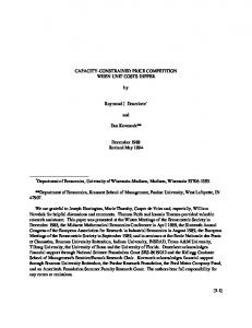
2 Problem formulation We consider the simple production-inventory system in Figure 1.

Insert Figure 1 Production-inventory system

The inventory is facing Poisson demand and is replenishing from production according to an S policy, i.e., there are no setup costs that motivate batch-ordering.

Fo

However, the production system can only process a single unit at a time, so it is not possible to have more than one order in process. If the inventory position is strictly

rP

less than S an order for one unit is triggered. Production is started as soon as the production of possible preceding units is finished. If there is no unit in production,

ee

production is started immediately. Production times are independent stochastic variables following a gamma distribution. The gamma distribution has several advantages in this context. The production time is always positive and we can fit the

rR

distribution to any mean and variance. Furthermore the demand during the stochastic production time will get a negative binomial distribution, which is easy to deal with.

ev

(See Section 3.2.) The gamma distribution is available in various software packages, e.g., in Excel. See Tijms (1994) for a comparison with other distributions.

iew

Components and/or raw materials needed in production can be obtained without any delay. Consequently, there are no holding costs associated with a unit before the production starts. Evidently, each unit produced incurs holding costs corresponding to the stochastic production time. However, the average holding cost in production for

On

an item is clearly independent of the ordering policy. We shall therefore disregard this holding cost. We consider, however, standard linear holding and backorder costs associated with time in inventory and customer waiting time.

ly

1 2 3 4 5 6 7 8 9 10 11 12 13 14 15 16 17 18 19 20 21 22 23 24 25 26 27 28 29 30 31 32 33 34 35 36 37 38 39 40 41 42 43 44 45 46 47 48 49 50 51 52 53 54 55 56 57 58 59 60

Page 4 of 12

At this stage we assume that the distributions of the stochastic production time and the demand are given. Our problem is then to choose the order-up-to level S in order to minimize the sum of expected holding and backorder costs.

We introduce the following notation: λ = intensity of the Poisson demand,

http://mc.manuscriptcentral.com/tprs Email: [email protected]

Page 5 of 12

3 µ = average production time per unit, σ = standard deviation of the production time per unit, ρ = λµ = traffic density, c = σ/µ = coefficient of variation for the production time, h = holding cost per unit and unit time, b = backorder cost per unit and unit time, S = order-up-to level, C = expected costs per unit of time.

Fo

Evidently we must require that ρ = λµ < 1. The gamma distribution that characterizes

rP

the production time for a unit is completely specified by the two parameters µ and σ.

ee

3 Cost evaluation and optimization 3.1

rR

The gamma distribution

Let us first for completeness define the gamma distribution, which has the density

(1)

iew

ξ(ξx ) r −1 e − ξx g( x ) = , x ≥ 0. Γ( r )

ev

The two parameters r and ξ are both positive and Γ(r) is the gamma function

∞

Γ(r ) = ∫ x r −1e −x dx . 0

(2)

ly

On

1 2 3 4 5 6 7 8 9 10 11 12 13 14 15 16 17 18 19 20 21 22 23 24 25 26 27 28 29 30 31 32 33 34 35 36 37 38 39 40 41 42 43 44 45 46 47 48 49 50 51 52 53 54 55 56 57 58 59 60

International Journal of Production Research

Given µ and σ the parameters r and ξ are uniquely determined as

r = (µ / σ) 2 ,

(3)

ξ = µ / σ2 .

(4)

It is useful to note that Γ(r) = (r-1)Γ(r-1) and that

http://mc.manuscriptcentral.com/tprs Email: [email protected]

International Journal of Production Research

4 ∞

∫x

α −βx

e

dx =

0

Γ(α + 1) , β (α +1)

(5)

for α > - 1 and β > 0.

3.2

Distribution of the demand during the production time

Next we consider the stochastic demand during the stochastic production time. The

Fo

demand process and the stochastic production time are independent. Let qj be the probability for demand j. We obtain

rP

∞

ξ(ξx ) r −1 e − ξx (λx ) j e − λx qj = ∫ dx . Γ(r ) j! 0

Using (5) we get

ξr q0 = , (λ + ξ) r

ξr λj r (r + 1)...(r + j − 1) . j! ( λ + ξ) r ( λ + ξ) j

ly

qj =

(8)

On

and for j > 0,

iew

i.e., for j = 0 we obtain

(7)

ev

(ξ) r λj Γ(r + j) , Γ(r ) j! (λ + ξ) r + j

rR

qj =

(6)

ee

1 2 3 4 5 6 7 8 9 10 11 12 13 14 15 16 17 18 19 20 21 22 23 24 25 26 27 28 29 30 31 32 33 34 35 36 37 38 39 40 41 42 43 44 45 46 47 48 49 50 51 52 53 54 55 56 57 58 59 60

Page 6 of 12

(9)

This means that qj has a negative binomial distribution that is easy to deal with. When, for a given µ, σ approaches 0, the distribution in (8) and (9) will, as expected, approach a Poisson distribution. However, for σ = 0, or σ very small, it is then computationally much more efficient to replace (8) and (9) by the Poisson distribution, i.e., to set

http://mc.manuscriptcentral.com/tprs Email: [email protected]

Page 7 of 12

5

qj =

(λr / ξ) j e − λr / ξ (λµ ) j e − λµ = . j! j!

(10)

Recall that we have defined the traffic density ρ = λµ, and the coefficient of variation for the production time c = σ/µ. The distribution qj in (9) is expressed in terms of three parameters λ, µ, and σ. However, it is easy to see that it can be specified completely by the two parameters ρ and c. Just note that λ/ξ = ρc2 and r = 1/c2.

The associated queuing system

rP

3.3

Fo

Note now first that the optimal solution must have S ≥ 0. Clearly, any S ≤ 0 will give zero holding costs. Furthermore, S < 0 must give higher backorder costs than S = 0.

ee

Assume then that we start with S items in stock. It is obvious that each demand will

rR

trigger a corresponding production order to be produced as soon as all previous orders have been produced. The orders in production or waiting to be produced constitute a so-called M/G/1 queuing system, i.e., we have Poisson arrivals and a production time

ev

that is not exponential. Using a standard approach we can derive the steady-state distribution for the queue length. See e.g., Grimmett and Stirzaker (1987) for details.

iew

Consider the number of waiting orders when an order has just been finished and delivered to inventory. If there are k orders waiting we say that the state of the queuing system is k. Let

On

pj = steady-state probability that the state is k (0, 1, 2, ....). First we have

ly

1 2 3 4 5 6 7 8 9 10 11 12 13 14 15 16 17 18 19 20 21 22 23 24 25 26 27 28 29 30 31 32 33 34 35 36 37 38 39 40 41 42 43 44 45 46 47 48 49 50 51 52 53 54 55 56 57 58 59 60

International Journal of Production Research

p0 = 1 - λµ = 1 - ρ,

(11)

i.e., the ratio of time when no production is taking place. To see this note that λµ is the average production time during a time unit. Consequently, 1 - λµ is the ratio of time when no production is going on. Next we note that

http://mc.manuscriptcentral.com/tprs Email: [email protected]

International Journal of Production Research

6

j+1

p j = p 0 q j + ∑ p i q j−i+1 ,

(12)

i =1

i.e., if we are in state 0 the next production concerns an order triggered by the next demand, but if the state is i > 0 the next production concerns one of the waiting orders.

Fo

Reformulating (12) we get

p j+1 =

1 q0

rP

j   p p q − −  j 0 j ∑ p j q j−i +1  i =1  

j = 0, 1, 2, ...

(13)

ee

i.e., we can easily determine the steady-state distribution recursively. Evidently pj → 0 as j → ∞ because ρ < 1. (In (13) the sum is defined to be zero for j = 0.)

rR

We note that p0 only depends on ρ. Because qj depends only on the parameters ρ and

ev

c this must then be the case also for all pj.

iew

Let us conclude at this stage that it is very easy to determine the steady-state distribution of the number of outstanding orders. The distribution is completely specified by the parameters ρ and c. First we get the distribution of the demand during

On

the production time from (8) and (9). Then we simply apply (11) and (13). Note that the distribution of the number of outstanding orders is independent of S.

3.4

Evaluation of costs and optimization of S

ly

1 2 3 4 5 6 7 8 9 10 11 12 13 14 15 16 17 18 19 20 21 22 23 24 25 26 27 28 29 30 31 32 33 34 35 36 37 38 39 40 41 42 43 44 45 46 47 48 49 50 51 52 53 54 55 56 57 58 59 60

Page 8 of 12

We are now ready to evaluate the expected costs for a given S ≥ 0. If there are k outstanding orders, the inventory level is S – k. Consequently, the expected costs for a given S can be expressed as ∞

[

]

C = ∑ p k (S − k ) + h + (S − k ) − b , k =0

http://mc.manuscriptcentral.com/tprs Email: [email protected]

(14)

Page 9 of 12

7 where x+ = max (x, 0) and x- = max (-x, 0).

It is easy to see that C is a convex function of S. Consequently, to find the optimal solution we simply evaluate S = 0, 1, ... The first local optimum is also the global optimum.

4 Numerical results and discussion We have shown that the optimal policy and the optimal costs (for given holding and

Fo

backorder costs) only depend on the traffic density ρ and the coefficient of variation c. So, for example, λ = 1, µ = 0.8, and σ = 0.4 give exactly the same results as λ = 10,

rP

µ = 0.08, and σ = 0.04, because in both cases ρ = 0.8 and c = 0.5. Furthermore, concerning the costs it is obvious that it is only the ratio between the backorder cost b

ee

and the holding cost h that is of interest. If both costs are changed by a certain percentage, this will change the optimal costs by the same percentage but the optimal

rR

policy is not affected. Therefore, in our numerical study we assume that h =1. Two different values of the backorder cost b = 5 and b = 20 are considered in Table 1 and Table 2 respectively.

Optimal policies and costs for h = 1 and b = 5.

iew

Insert Table 1

ev

ly

On

1 2 3 4 5 6 7 8 9 10 11 12 13 14 15 16 17 18 19 20 21 22 23 24 25 26 27 28 29 30 31 32 33 34 35 36 37 38 39 40 41 42 43 44 45 46 47 48 49 50 51 52 53 54 55 56 57 58 59 60

International Journal of Production Research

http://mc.manuscriptcentral.com/tprs Email: [email protected]

International Journal of Production Research

8

Insert Table 2

Optimal policies and costs for h = 1 and b = 20.

In both tables we have evaluated the costs for the same four values of ρ and five values of c. It is not surprising that the costs will increase both with ρ and c. From the tables it is also obvious that the additional cost when increasing c is much larger when ρ is high, and similarly the additional cost when increasing ρ is much larger when c is high. All such tendencies are stronger with the higher backorder cost in Table 2.

Fo

We believe that our simple model may be useful in connection with evaluation of

rP

investments in production. Such an investment will in general reduce the average production time µ and also the standard deviation of the production time σ. Clearly

ee

this means that ρ is reduced. The coefficient of variation c may both decrease and increase. If, for example, µ and σ are reduced by the same percentage, this means that

rR

c is unchanged. Our model shows how the inventory costs are affected by the investment. If µ is reduced we will also get lower holding costs for the time in production. These costs are normally proportional to 1/µ and easy to evaluate. The

ev

total reduction of holding and backorder costs should then be compared to the cost for a considered investment.

5 Conclusions

iew

We have suggested a simple model of a production-inventory system. The demand is

On

Poisson and the production time for a unit is modeled as a gamma distributed stochastic variable. The system is controlled by a so-called S policy. Using M/G/1 queuing theory it is very easy to evaluate and optimize holding and backorder costs,

ly

1 2 3 4 5 6 7 8 9 10 11 12 13 14 15 16 17 18 19 20 21 22 23 24 25 26 27 28 29 30 31 32 33 34 35 36 37 38 39 40 41 42 43 44 45 46 47 48 49 50 51 52 53 54 55 56 57 58 59 60

Page 10 of 12

which only depend on the traffic density and the coefficient of variation for the production time.

The considered model may be useful when evaluating different investments in the production system, because such investments will, in general, affect holding and backorder costs in a way that is easy to illustrate by our model.1

1

I am grateful to Christian Howard for help with parts of the numerical evaluation.

http://mc.manuscriptcentral.com/tprs Email: [email protected]

Page 11 of 12

9

References Axsäter, S. 1980. Economic Order Quantities and Variations in Production Load, International Journal of Production Research, 18, 359-365. Axsäter, S. 2006. Inventory Control, 2nd edition, Springer, New York. Geng, N., and Z. Jiang. 2009. A Review on Strategic Capacity Planning for the Semiconductor Manufacturing Industry, International Journal of Production Research, 47, 3639-3656.

Fo

Grimmett, G. R., and D. R. Stirzaker. 1987. Probability and Random Processes, Oxford University Press, New York.

rP

Jönsson, H., and E. A. Silver. 1985. Impact of Processing and Queuing Times on Order Quantities, Material Flow, 2, 221-230.

ee

Karmarkar, U. S. 1987. Lot Sizes, Lead Times and In-Process Inventories, Management Science, 33, 409-418. Karmarkar, U. S. 1993. Manufacturing Lead Times, Order Release and Capacity Loading, in S. C. Graves et al. Eds. Handbooks in OR & MS Vol. 4, North Holland Amsterdam, 287-329.

ev

rR

Pac, M. F., Alp, O., and T. Tan. 2009, Integrated Workforce Capacity and Inventory Management under Labour Supply Uncertainty, International Journal of Production Research, 47, 4281-4304.

iew

Tijms, H. C. 1994. Stochastic Models: An Algorithmic Approach, Wiley, Chichester. Vits, J., Gelders, L., and L. Pintelon. 2007. Manufacturing Process Changes: Myopic and Long-term Planning, International Journal of Production Research, 45, 1-28.

On

Zipkin, P. H. 1986. Models for Design and Control of Stochastic, Multi-Item Batch Production Systems, Operations Research, 34, 91-104. Zipkin, P. H. 2000. Foundations of Inventory Management, McGraw-Hill, Singapore.

ly

1 2 3 4 5 6 7 8 9 10 11 12 13 14 15 16 17 18 19 20 21 22 23 24 25 26 27 28 29 30 31 32 33 34 35 36 37 38 39 40 41 42 43 44 45 46 47 48 49 50 51 52 53 54 55 56 57 58 59 60

International Journal of Production Research

http://mc.manuscriptcentral.com/tprs Email: [email protected]

International Journal of Production Research

Production system

Inventory

Figure 1 Production-inventory system

Table 1

Fo

Optimal policies and costs for h = 1 and b = 5. c=0

ρ = 0.9

ρ = 0.7

11 10.77 5 5.18 3 3.33 2 2.41

c=1

c = 1.5

c=2

17 17.01 8 8.03 5 5.02 3 3.44

26 27.37 12 12.71 7 7.74 4 5.19

40 41.89 17 19.26 10 11.57 6 7.61

Table 2

ρ = 0.8

ρ = 0.6

S C S C S C S C

c=0

c = 0.5

c=1

c = 1.5

c=2

15 14.74 7 7.15 5 4.65 3 3.41

18 18.28 9 8.78 6 5.65 4 4.00

28 28.89 13 13.62 8 8.49 5 5.95

45 46.56 21 21.70 12 13.30 8 9.02

69 71.29 31 32.98 18 20.01 12 13.39

ly

ρ = 0.7

Optimal policies and costs for h = 1 and b = 20.

On

ρ = 0.9

iew

ev

rR

ρ = 0.6

8 8.69 4 4.25 3 2.77 2 2.02

ee

ρ = 0.8

S C S C S C S C

c = 0.5

rP

1 2 3 4 5 6 7 8 9 10 11 12 13 14 15 16 17 18 19 20 21 22 23 24 25 26 27 28 29 30 31 32 33 34 35 36 37 38 39 40 41 42 43 44 45 46 47 48 49 50 51 52 53 54 55 56 57 58 59 60

http://mc.manuscriptcentral.com/tprs Email: [email protected]

Page 12 of 12